Detection of transient sub-pockets in crystal structures
As an example we will use p38 MAP kinase
1. Overview:
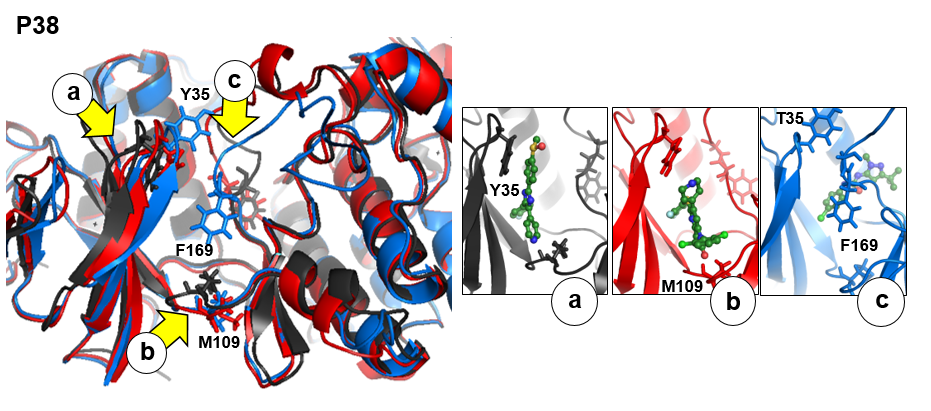
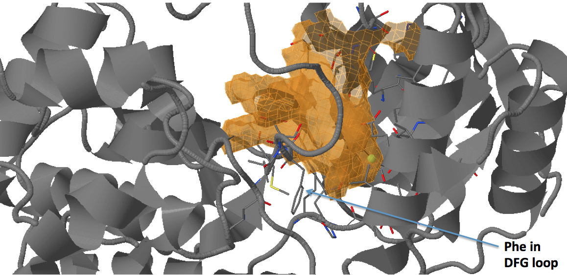
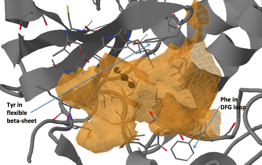
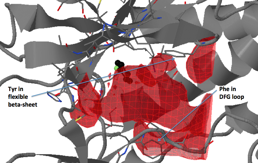
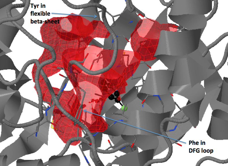
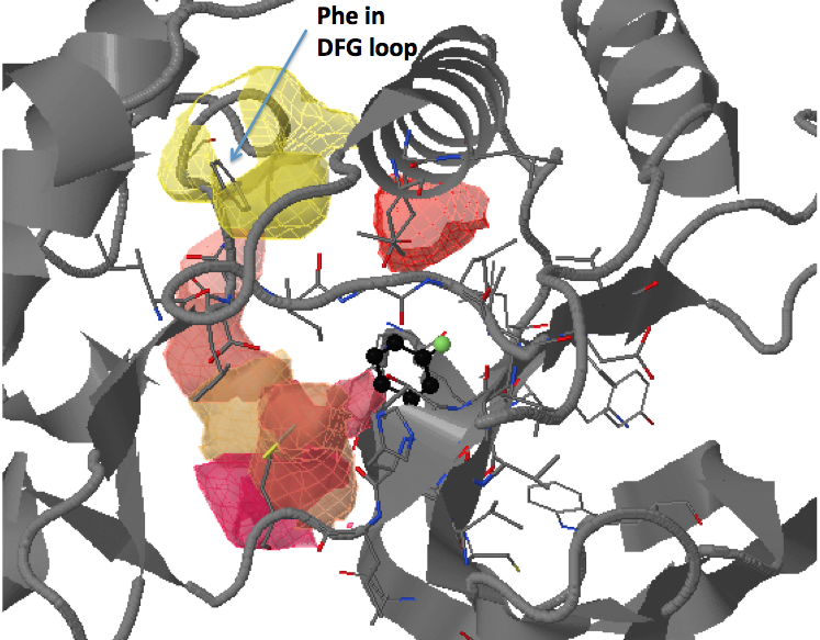
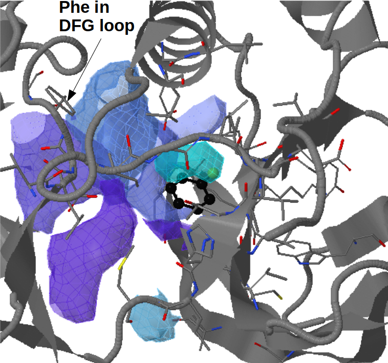
There are three transient pockets (a, b, and c, see Fig.1) that arise from the motion of the beta-sheet (ATP-binding site, denoted as a), reorganization of the activation loop containing the highly conserved Asp-Phe-Gly (DFG) motif (c), and flipping of the M109 residue with small backbone shifts (b). Sub-pocket c is closed in crystal structures 1a9u and 1ouy but open in the crystal structure 1kv1.
The activation loop (residues above the DFG loop with numbers between 170 and 185) is missing in many structures where the transient sub-pocket C behind the DFG loop is open (inactive state II). The missing residues do not contribute to the binding site.
2. To run these examples, you need the following files and parameters:
- prot.pdb The reference structure (generated by grep ATOM 1a9u.pdb > prot.pdb from the 1a9u pdb file)
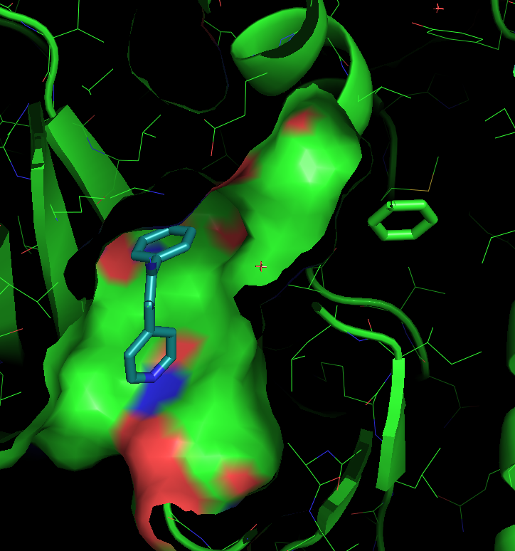
- ligand.pdb The ligand that will be used for defining the binding site. As the ligand, we use just one ring of the ligand in the PDB 1a9u structure, that is positioned at about the pocket center.
- 17 PDB structures of the protein extracted from the archive PDB_structures.tar
Since we know that some residues that are in the vicinity of the binding site are missing in some structures, we use a relatively small pocket radius to be sure that the binding site is complete. Taking into account, that our ligand is defined as one aromatic ring, we set pocket radius = 8 Angstroms.

3. Simulation procedure and results
- Step 1: Uploading reference structure and defining input parameters
You have to upload the reference structures of the protein and ligand and click Upload trajectories at the next step before you go to the Next Step.
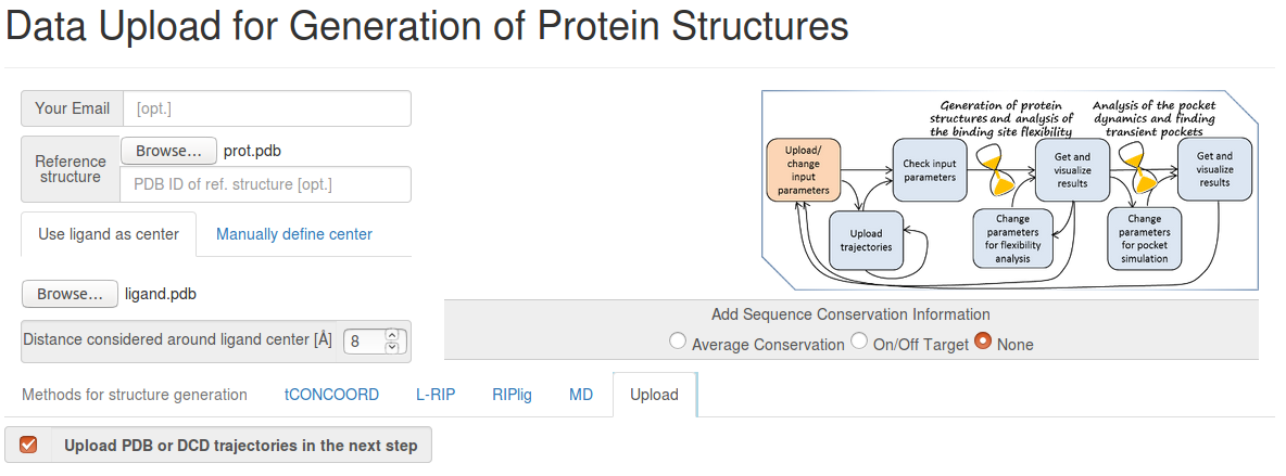
- Step 2: Uploading PDB structures
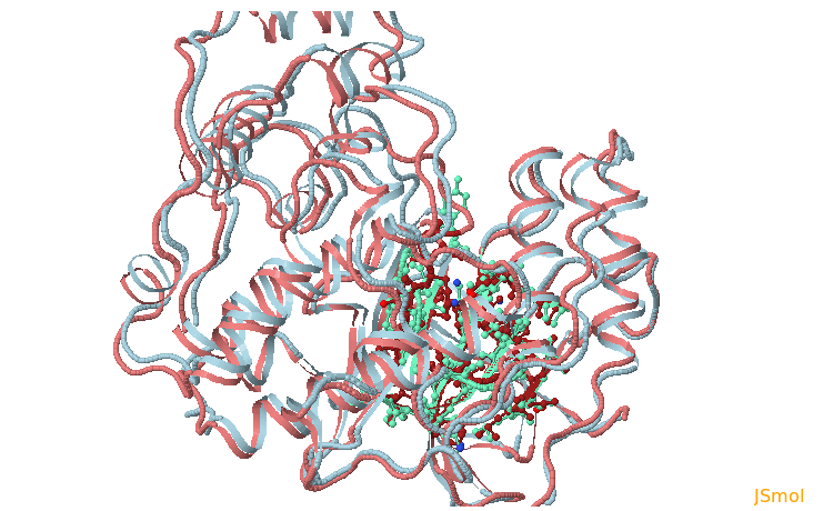
In the next page Pocket analysis will be started with the following parameters you must be able to see the JSmol visualization of the reference structure and an identified binding pocket. You can then upload all PDB structures (as PDB trajectories) sequentially and launch TRAPP-structure/analysis. Since no method for generation of new structures was selected in the previous step, only analysis of the uploaded structures (trajectories) will be done.
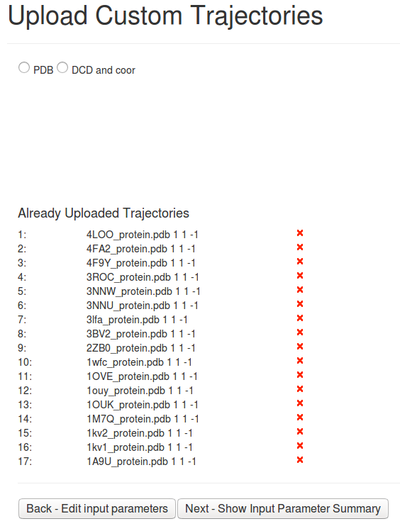
- Step 3 : Checking input data and starting simulations
On the page Upload Custom Trajectories: Check if a list of PDB files at the bottom of the page contains all structures you want to analyze. Then click Launch TRAPP structure/analysis.

- Step 4: Viewing simulation results of TRAPP-analysis
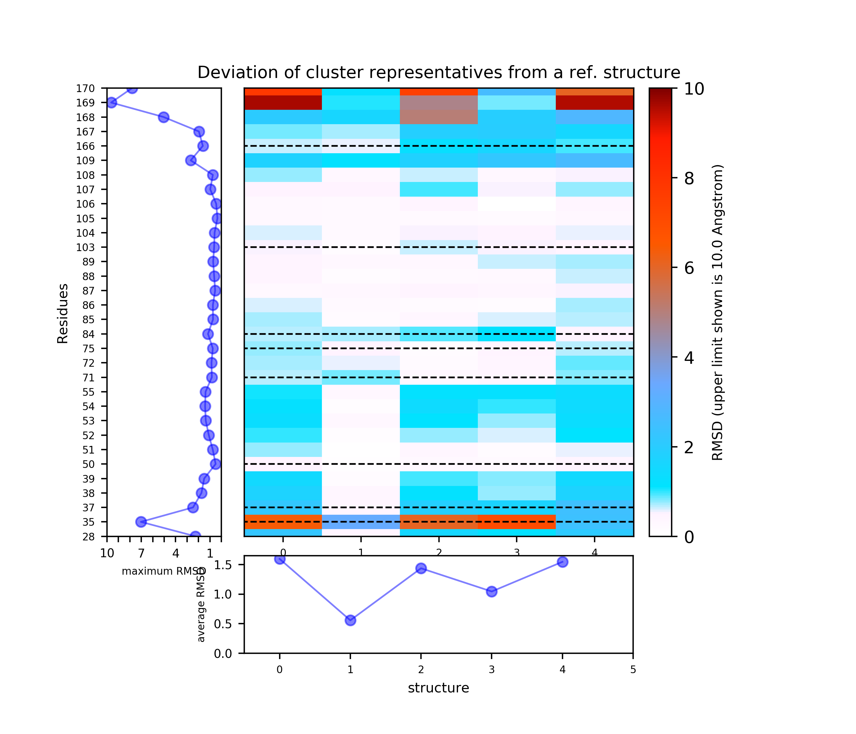
When the job is completed you can open a page with preliminary results (link View Analysis). Note that TRAPP-analysis runs in this step with default parameters (backbone atoms are used for RMSD calculations and a fast hierarchical clustering of the binding site conformations is carried out with a threshold of 3 Angstroms).
These parameters may not be well suited to our particular case. Specifically, selected binding site residues may not completely represent the binding pocket, or, alternatively, may include residues that are not related to the binding site regions (use the link View cluster representatives in JSmol for a view of selected binding site residues that are shown by sticks). This can be corrected by changing parameters and clicking re-run TRAPP-analysis. Look in the Log_file to see if any residues in the binding pocket are missing (for example, the line TRAPP:------trj: 165LEU(ref: 166PHE) -> mutated means that PHE166 is probably absent in your PDB structure and instead the next residue will be used for alignment and RMSD calculations)

- Step 5: Re-run TRAPP-analysis using k-means clustering
We add residues 166, 169 and 170 (particularly, Phe169 in original PDB structure, from the DFG loop) to the list and residue 28 from the flexible beta-sheet (transient pocket A).
We also choose k-means clustering, and increase RMSD to be used for preliminary hierarchical clustering of structures to 5 Angstroms in order to reduce the number of clusters. We also increase Maximum value of deviation to be shown in plots to 10 Angstroms. Then click Re-run TRAPP-analysis (Note the binding site residues are renumbered as shown in the residue mapping and summary input page).
Binding site motions were found around residues 165-167 (DFG and part of the activation loop) and residues 32-33 (beta-sheet motion).(Note the binding site residues are renumbered as shown in the residue mapping and summary input page, in this example by 3 residues).

- Step 6: Editing TRAPP-pocket parameters and running TRAPP-pocket
- Check Use TRAPP-analysis based binding site residues: To make sure that all binding site residues are included in pocket simulations.
- Check H-atoms to be generated for the reference structure and H-atoms to be generated for structures in trajectories to ensure correct pocket shape. There is another (faster, but less accurate) method of taking into account hydrogen atoms in pocket calculations by increasing the Lennard-Jones radii used for pocket identification (for this, uncheck Calculate Druggability then check Only heavy atoms to be used in Define pocket position and grid size for the pocket identification procedure).
- Change Analysis will be done at the pocket occurrence of (%): to 6, 10, 12, 18, 30 (we have 17 structures, so 1 structure corresponds to 6% occurrence). Check run PCA and run Clustering.
- Check Calculate Druggability to make druggability prediction by applying the grid settings from the TRAPP-LR/CNN models that are trained on the bindability datasets.
- Launch TRAPP-pocket.
For our example the Trapp-pocket parameters are adjusted as follows:
- Step 7: Understanding TRAPP-pocket results
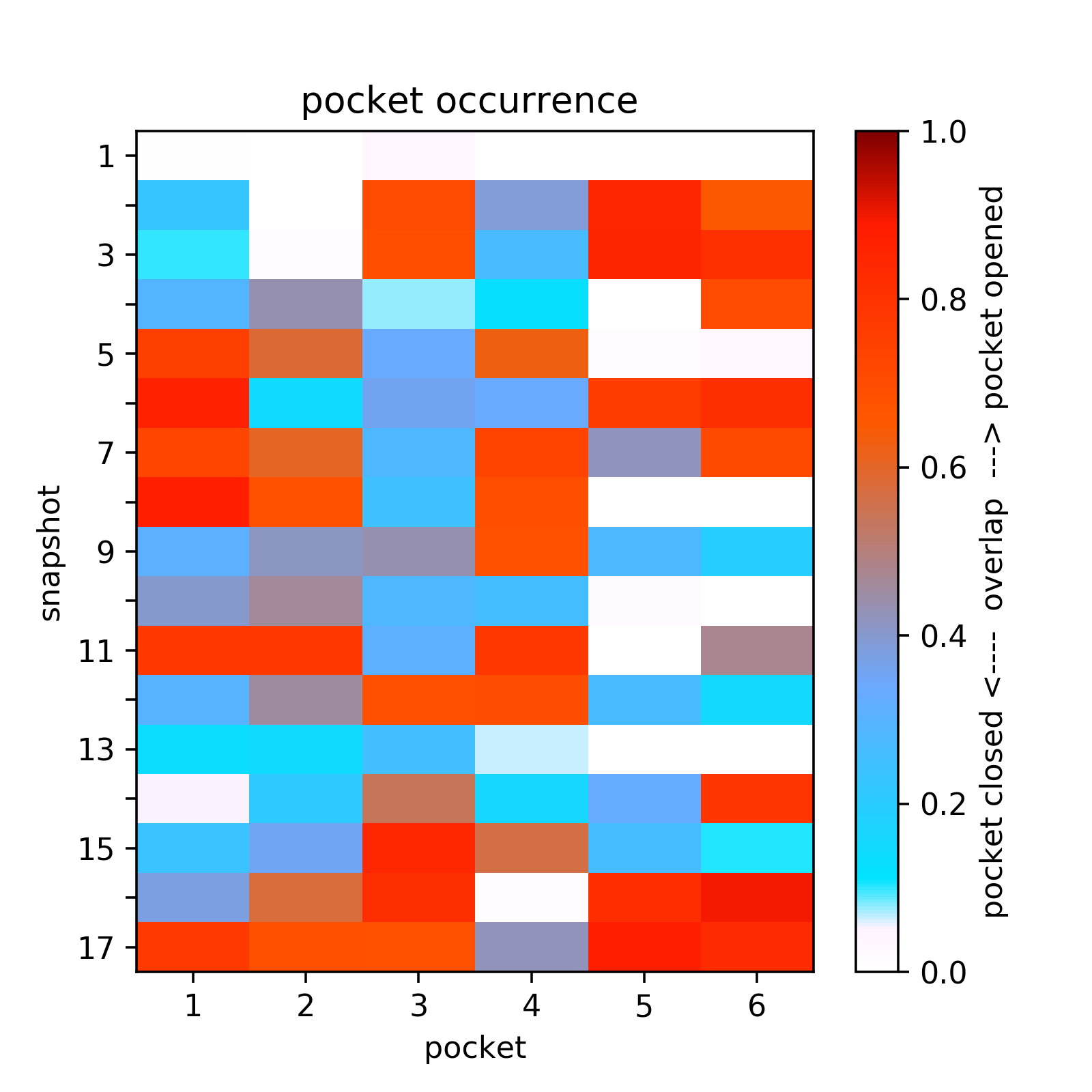
- Transient regions are shown at 20% occurrence, i.e. they are open in 3-4 structures (since we uploaded 17 structures).
- This, however, does not mean that all transient regions shown are open simultaneously in the snapshots.
- To find in which snapshot/structure a particular transient region is open, one has to use the tab Pocket Characteristics.
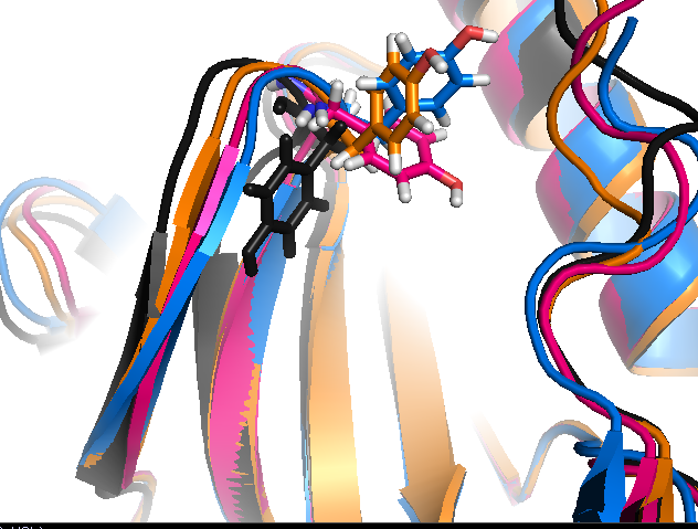
- Sub-pocket #2 arises from the motion of Y35 (sub-pocket A) and is mostly open in structures 3lfa, 1wfc, and 4f9y.
- The heatmap of the pocket occurence in the trajectory is shown in Fig.14. Use a link shown above the plot to get original data.
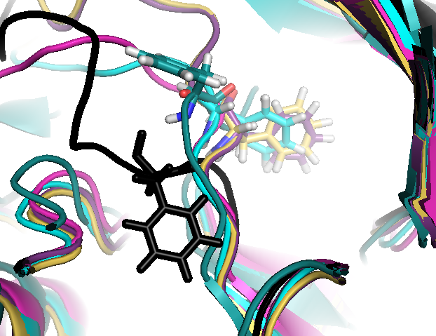
- Sub-pocket #6 corresponds to transient pocket C arising from motion of the DFG loop. They are mostly open (to different degrees) in 3nnw, 3nnu, 3roc,1kv2, and 1kv1. (See Fig.15 and 16)
The results of TRAPP-pocket simulations can be viewed using the link: "Combined trajectories" to an HTML file that uses JSmol for visualization of transient pockets.
Conserved/transient regions: yellow - pocket population (see Fig.11a and Fig.11b), red - transient pocket regions that are absent in the reference structure, but appear in some other structures. (See Fig.12a and Fig.12b)
Click Clustering of transient regions opening in a percentage of snapshots - 18%:
Here opening transient pocket regions are split into three pockets and
the largest one is split once more into sub-regions(sub-pockets). Appearing pockets are colored in red/yellowish and disappearing pockets in blue/purplish. (See Fig.13a and 13b)
- Step 8: Analyzing TRAPP-pocket druggability results
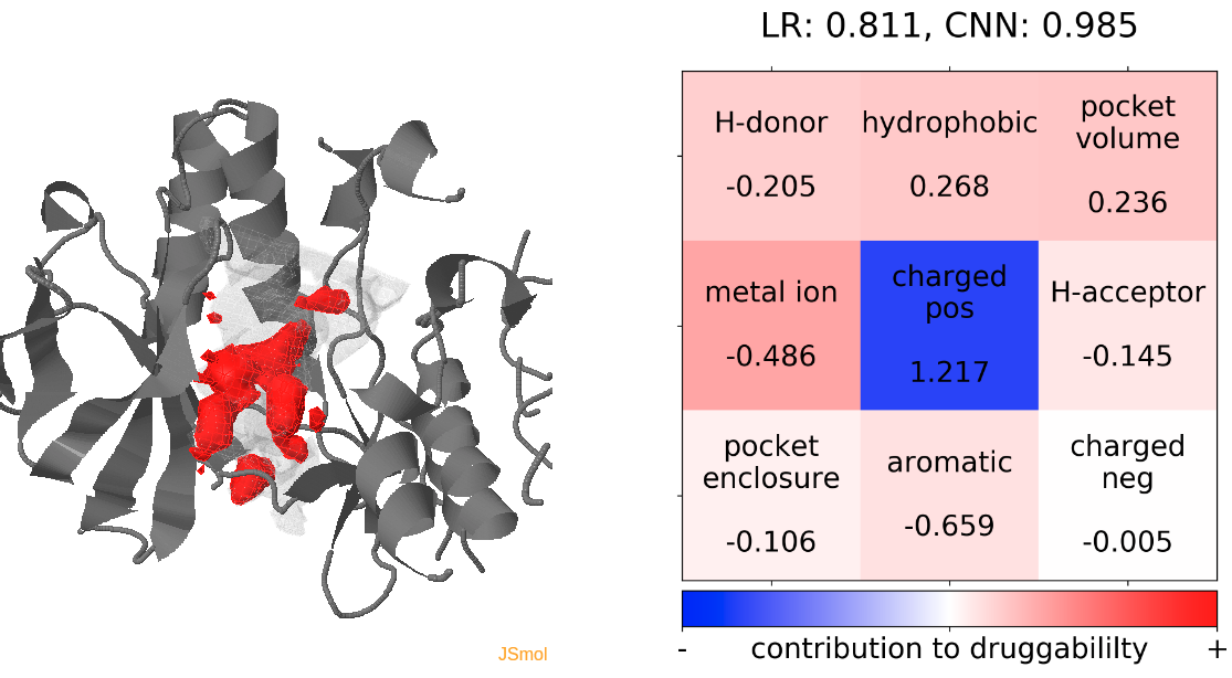
- Snapshot 0 refers to the pocket druggability data obtained from the reference structure. (See Fig.18)
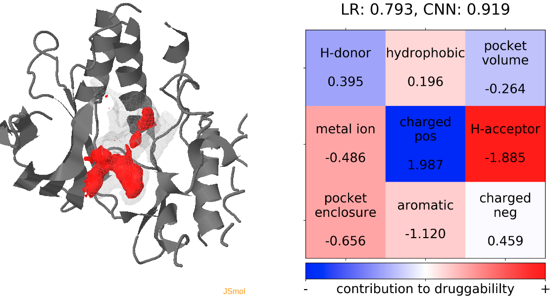
- The lowest druggability score is with the trajectories of the protein conformation from pdb 1wfc, where high number of positively charged residues seem to be a strong contributor to lower druggability score. (See Fig.19)
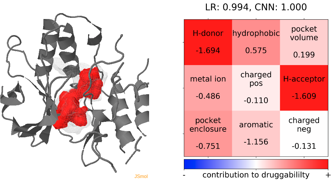
- The highest druggability score is with the trajectories of the protein conformation from pdb 1kv2. The absence of H donors and acceptors in the pocket and high hydrophobicity were the major contributors to high druggability. (See Fig.20)
The results of TRAPP-pocket druggability are available under the Pocket characteristic tab.
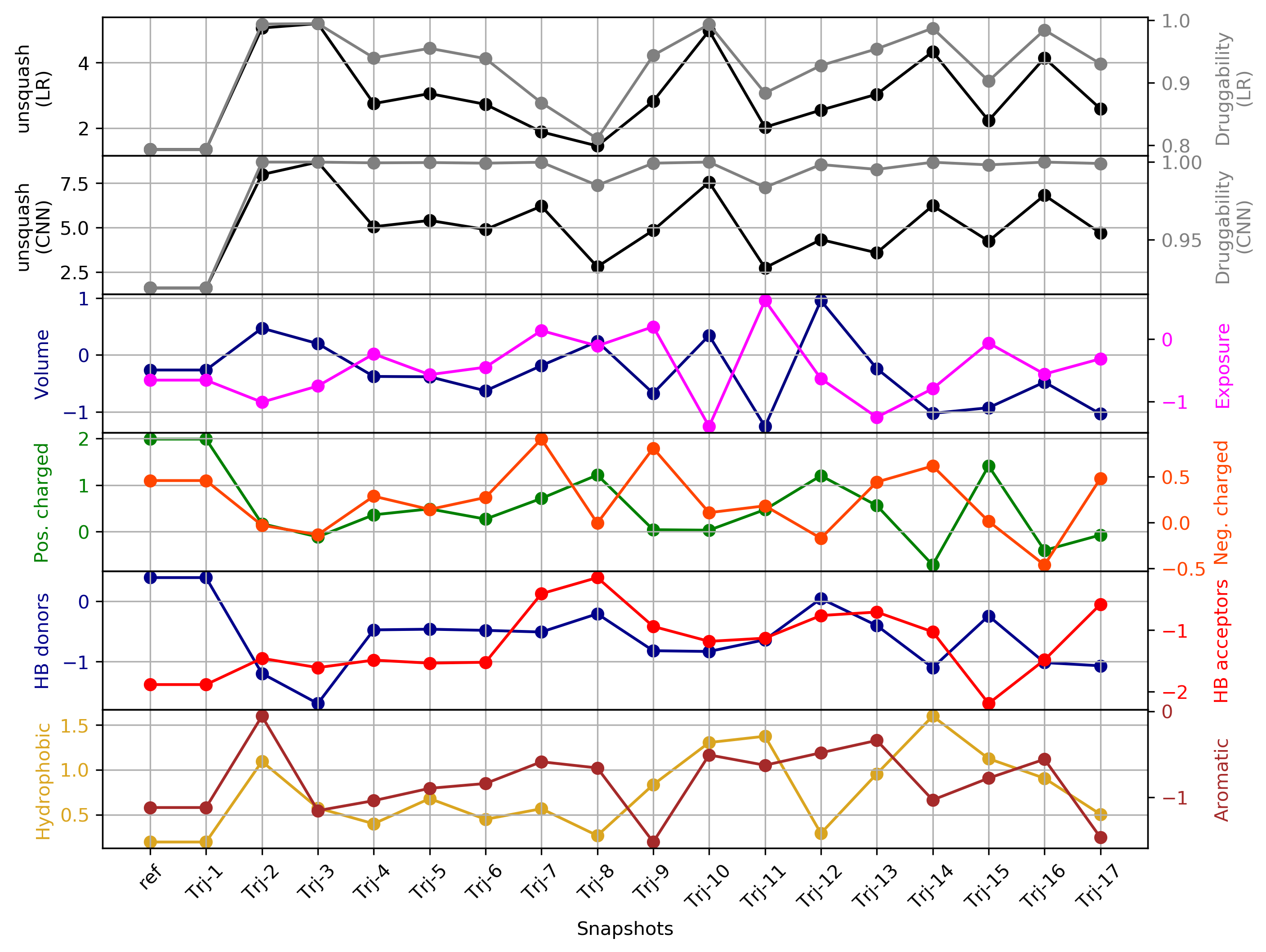
Click Pocket characteristics and druggability to visualize different physicochemical characteristics of the pocket and their contribution to the druggability (See Fig.17).
The druggability score of each cluster representative of the MD trajectories was predicted by both TRAPP-LR and TRAPP-CNN models. The pocket druggability for a specific cluster of the MD trajectories can be analyzed by choosing the respective snapshot and clicking Load Result in Druggability information for selected snapshot section.