Finding transient pocket regions in a molecular dynamics trajectory
In this example, a 6ns MD trajectory is used for identification of transient binding pockets in aldose reductase (AR)
1. Overview :
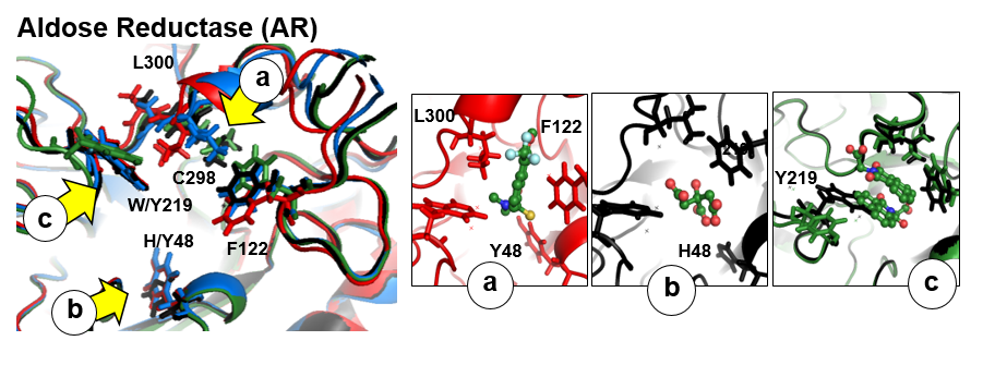
There are three flexible pocket regions in human AR denoted as a, b, and c. Sub-pocket a is occupied by tolrestat, TOL, and the inhibitor compound, IDD594, in crystal structures 1ah3 and 1us0, respectively; the ligand citric acid (CIT) occupies sub-pocket b in structure 2acu of the Y48H mutant of AR; the two molecules of the drug alrestatin, ALR, (both present in the crystal structure 1az1 of the C298A/W219Y mutant of AR) stack with each other with one occupying sub-pocket a and one occupying sub-pocket c (see Fig. 1). In this example , we will analyse a 6ns MD simulation of the Y48H mutant of human aldose reductase (AR)
2. To run this example, you need the following files and parameters:
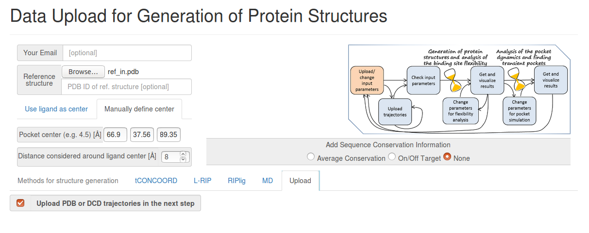
- Ref_in.pdb the reference structure (2acu pdb file, containing only the protein with H atoms added)
- Md.pdb a trajectory in PDB format that consists of 60 snapshots from an MD simulation (written at 100ps intervals)
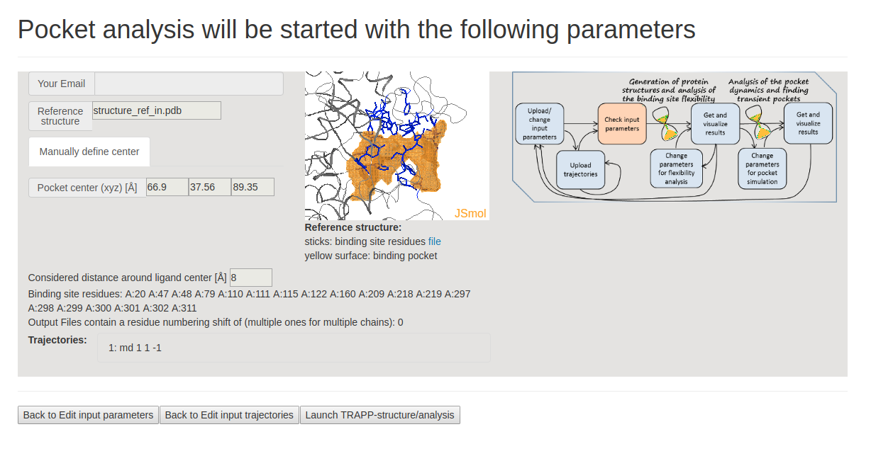
- Binding pocket center defined by x, y, z coordinates in Angstroms: 66.9, 37.56, 89.35
- Radius defined in Angstrom: 8
3. Simulation Procedure and Results
- Step 1: Uploading the reference structure and defining the input parameters
You have to upload the reference structure and to specify coordinates of the pocket center and the effective pocket radius (for this, choose Manually defined center).
You also have to click Upload PDB or DCD trajectories at the next step before you go to the Next Step (See Fig.2).
- Step 2: Uploading trajectories
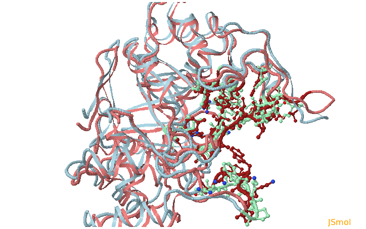
On the next page Pocket analysis will be started with the following parameters, you must be able to see a JSmol visualization of the reference structure and an identified binding pocket. You can then upload the trajectory (or trajectories) and launch TRAPP-structure/analysis. Since no method for generation of new structures was selected in the previous step, only analysis of the uploaded trajectory(or trajectories) will be done. (See Fig.3)
- Step3 : Checking input data and starting simulations
On the page titled Pocket analysis will be started with the following parameters: - Press the button Launch TRAPP structure/analysis.
- Step4: Viewing simulation results of TRAPP-analysis
When the job has completed you can open a page with the preliminary results of the TRAPP-analysis procedure. Note, that at this step the default parameters of the TRAPP-analysis are used (backbone atoms are used for RMSD calculations and a fast hierarchical clustering of the binding site conformations is carried out with a threshold of 3 Angstroms).
Use the link View Analysis to see a summary of the simulation results, which includes:
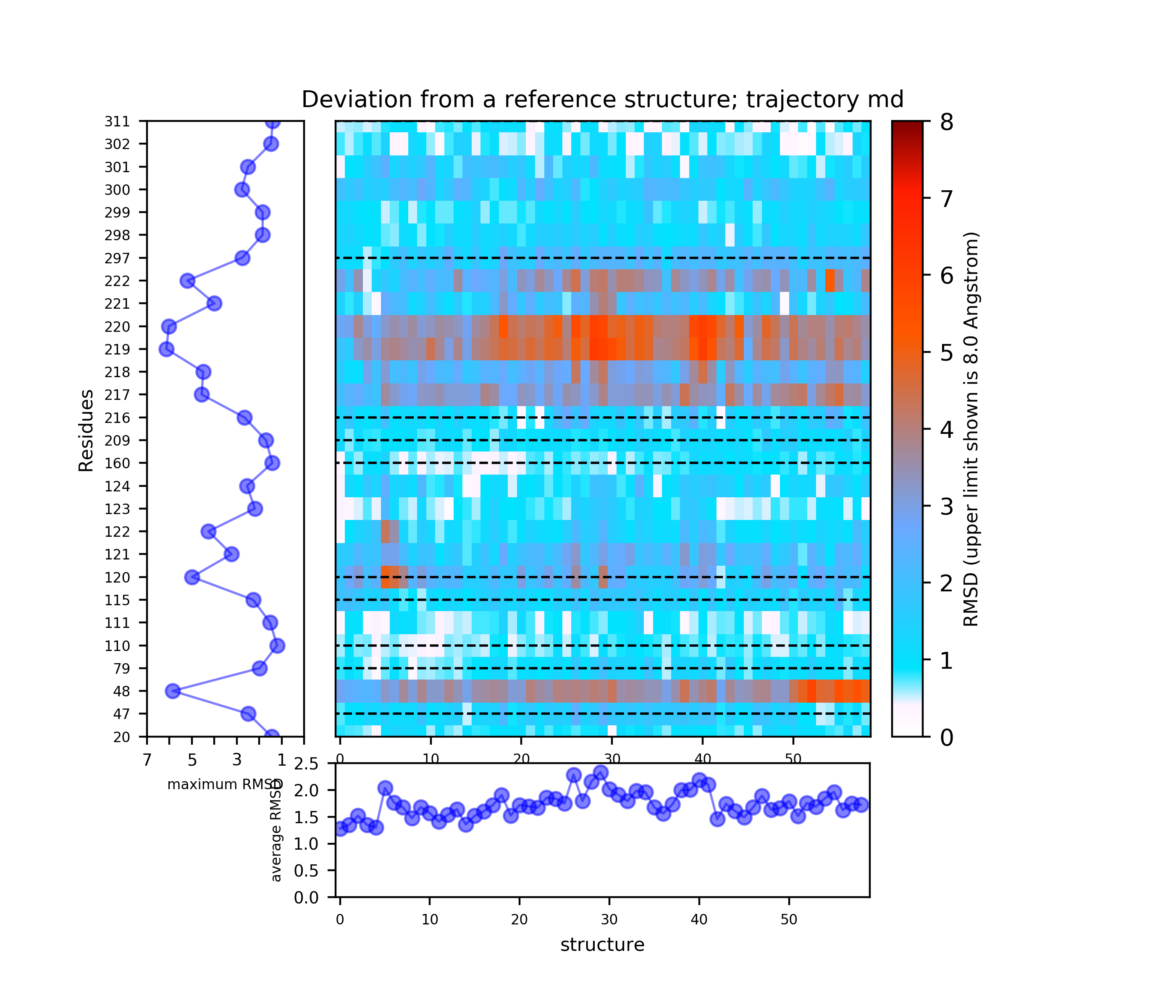
(i) A plot showing the RMS deviation of each residue from the reference structure in each snapshot of the trajectory (you can also download the data by clicking on the sign placed under the image). The regions of residues 218-219 and 122 are the most flexible with a deviation of up to 7 Angstroms from the reference structure. (see Fig.4)
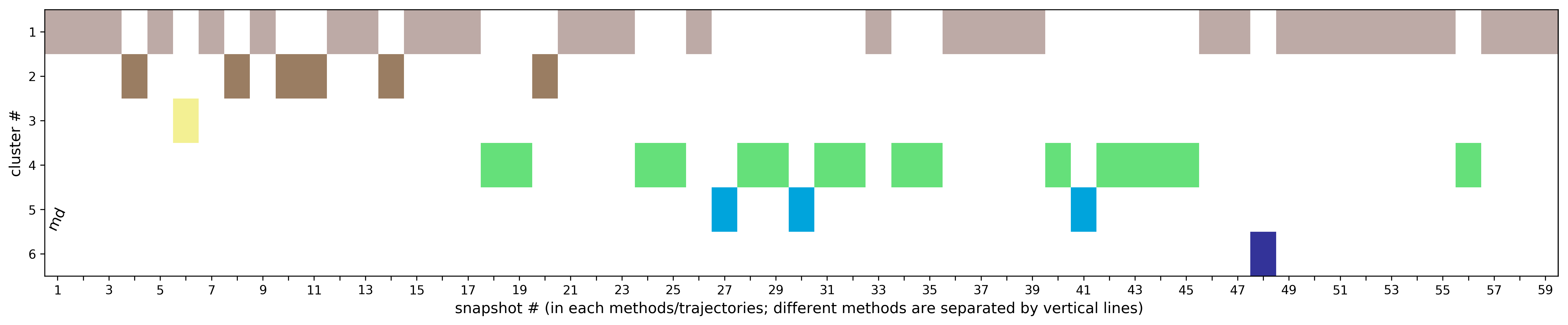
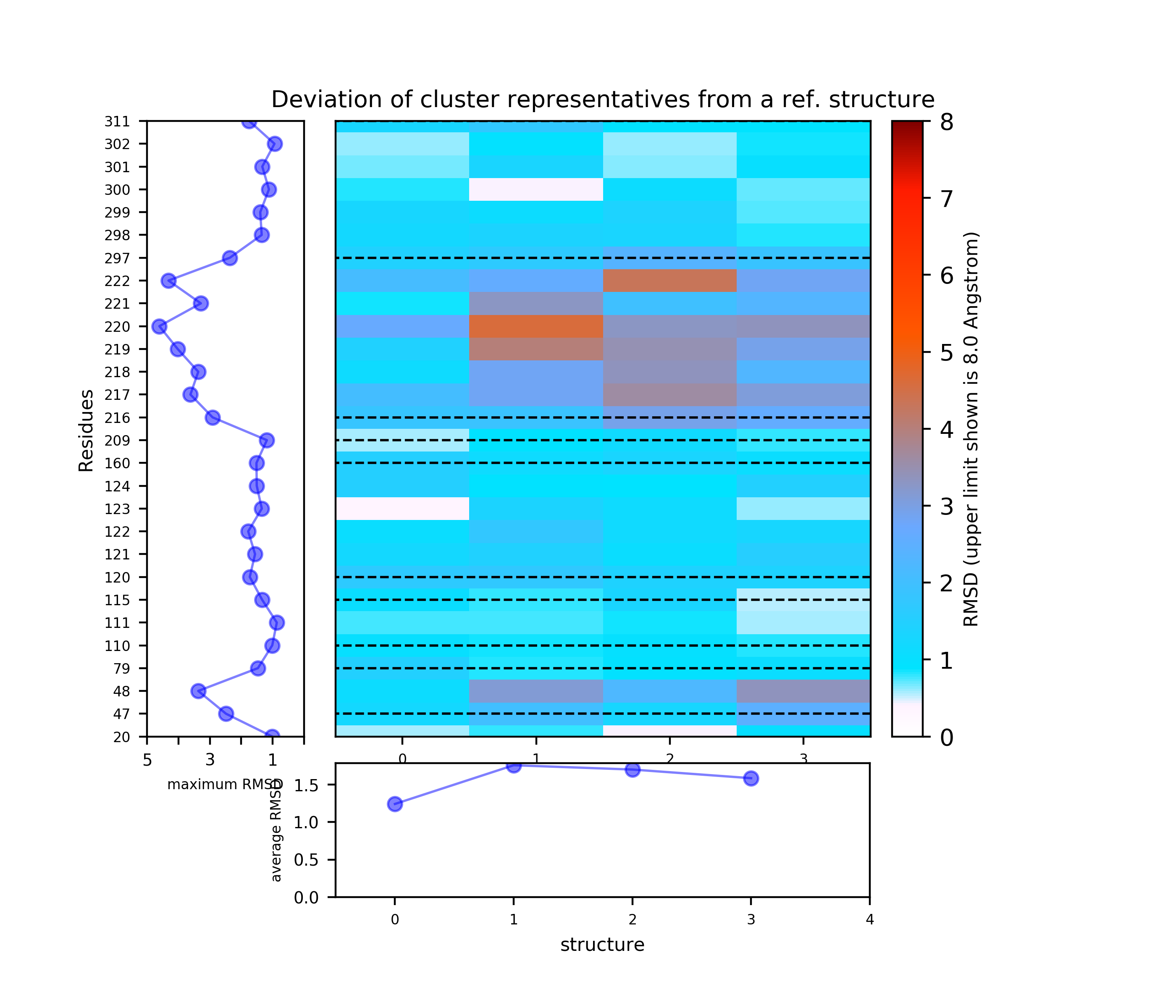
(ii) Clustering results: a distribution of snapshots over clusters. (See Fig.5 and Fig.6)
Using the link List of Cluster Representatives you can download PDB structures of cluster representatives.


- Step 5: Re-run TRAPP-analysis using k-means clustering
By choosing the button Re-run TRAPP-Analysis, you can change the parameters on the next page. In particular, you can run a more accurate clustering; use geometric centers of the binding site residues instead of only backbone atoms to compute RMSD; change RMSD in clusters; or include additional residues in the binding site list.
In this example, we add the residues 120, 121, 123, 124, 216, 217, 220, 221, and 222 to the binding site and choose k-means clustering.
The results will be found on the "View Analysis" link. Binding site motions were found around the residues 48 and 217-222 (corresponding to flexible regions B and C in the crystal structures) and around 120-122. The analysis was done using backbone atoms to compute the RMSD (See Fig.7 and Fig.9-12).
When geometric centers of residues are used for clustering (See Fig.8) some fluctuation of residues 300 and 301 (sub-pocket a) appears.


- Step 6: Running TRAPP-pocket and analyzing the simulation results
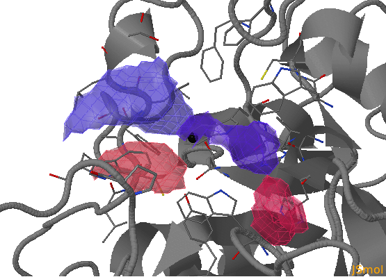
- sub-pocket b consists of opening (red) and closed (blue) parts relative to the reference structure that corresponds to changes in the position of H48 opening one pocket part and closing another.
- sub-pocket c appears due to a loop motion (W219).
In this example we click run PCA and run Clustering. Analysis will be done at the pocket occurrence of (%) of 10, 30, 65. Check the Calculate Druggability box to compute pocket druggability. Click Launch TRAPP-pocket to start.
The results of TRAPP-pocket simulations can be viewed using the link: USER-TRJ Results: Trj-md to an HTML file that uses JSmol for visualization of transient pockets. (View simulation result in JSmol )
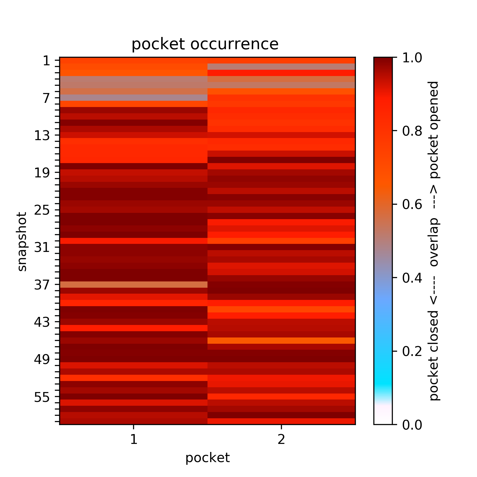
Two transient regions (B,C) are observed in at least 70 % of snapshots:Opening and closing of transient sub-pockets along the MD trajectory can be analyzed using the Pocket Characteristics tab.
Here all transient sub-pockets are split into separate pockets (that are not connect with each other) and the large pockets are once more split into compact sub-pockets, then they overlap between pockets in each snapshot and the transient sub-pocket is computed and represented as a matrix.
For example at a pocket occurrence of 65%, one can see that sub-pocket c is mostly open because the loop moves opening a pocket (pocket 2, second column in the overlap matrix). (See Fig.13)

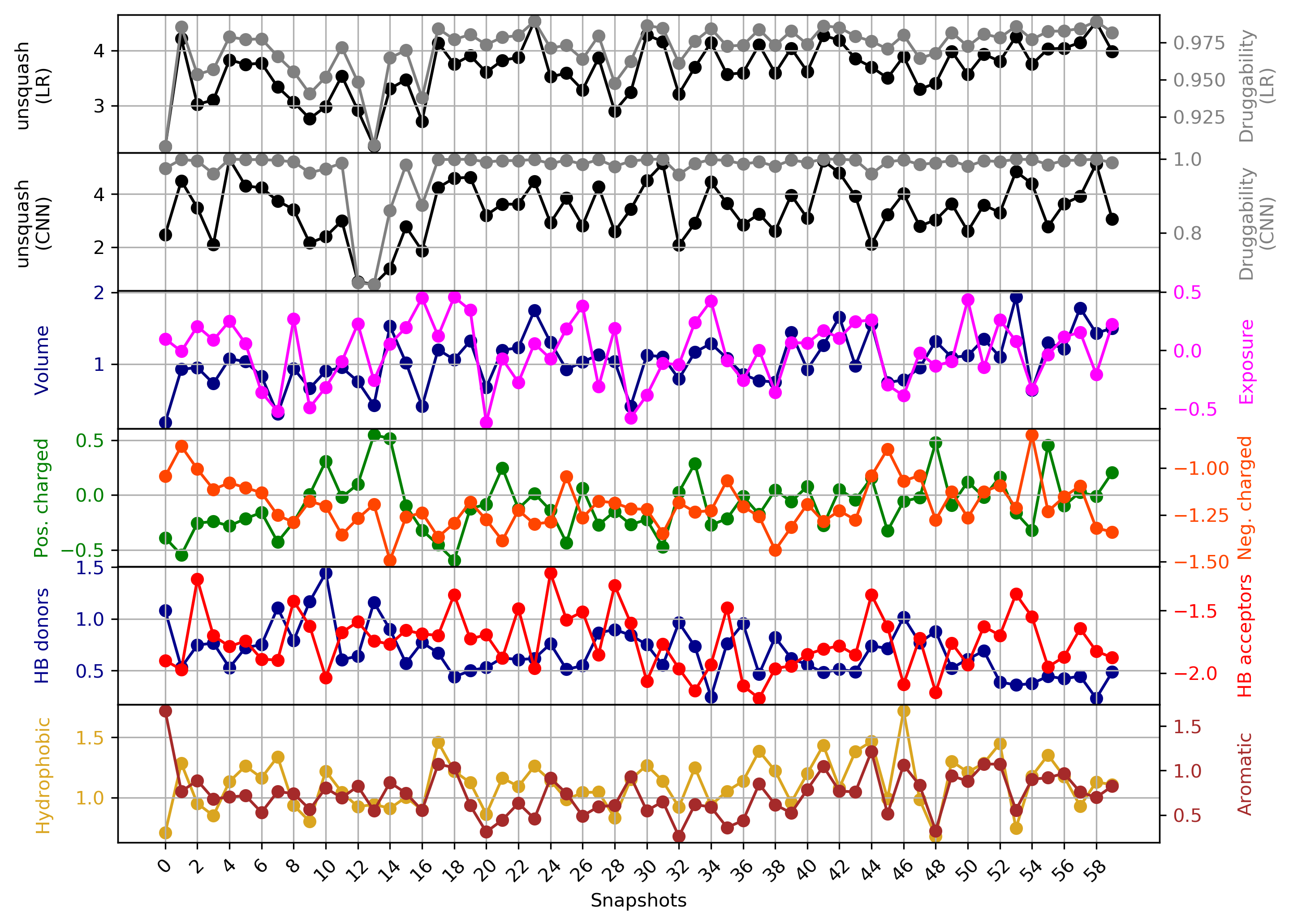
- Step 7: Analyzing TRAPP-pocket druggability results
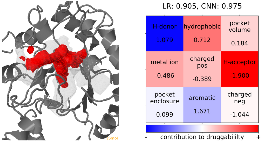
- Snapshot 0 refers to the pocket druggability data obtained from the reference structure. (See Fig.17)
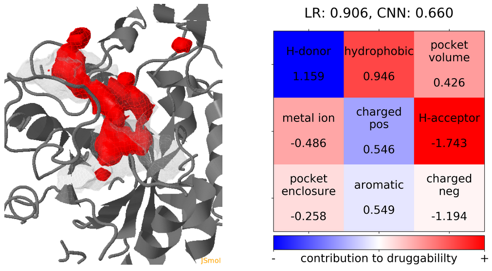
- The point with the lowest druggability score in the MD trajectory is at Frame 13, where more positively charged residues seem to be the reason for lower druggability (See Fig.18) when compared to the reference structure.
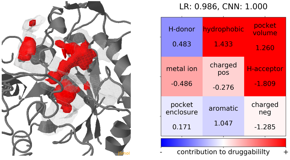
- The highest druggability score is at snapshot 41. The pocket volume, hydrophobicity of the pocket and the number of H-bond acceptors were the major contributors to druggability. (See Fig.19)
The results of TRAPP-pocket druggability are available under the Pocket characteristic tab.
Click Pocket characteristics and druggability to visualize different physicochemical characteristics of the pocket and their contribution to the druggability (See Fig.16).
The druggability score of each frame in the MD trajectory was predicted by both TRAPP-LR and TRAPP-CNN models. The pocket druggability at a specific point in the MD trajectory can be analyzed by choosing the respective snapshot and clicking Load Result in Druggability information for selected snapshot section.