TRAPP-Pocket workflow
Pocket tracking and identification of transient regions
- All structures are superimposed using the non-hydrogen atoms of the active site residues that are defined by the pocket center or the ligand position and a distance around the pocket center or the ligand (see input parameters).
- All snapshots of a trajectory are aligned and superimposed with the user-defined reference structure.
- The protein cavity distribution is calculated for each snapshot using the program (lj-pocket, described below) and saved in dx grid format. Additionally, detected pockets are represented by pseudo atoms for each snapshot. Snapshots are concatenated into a pdb trajectory that shows the motion of the protein cavities.
- Pocket dynamics are analyzed and transient/conserved regions identified.
- PyMol and JSmol scripts are generated.
Pocket tracking: program lj-pocket
Lj-pocket implements a grid-based procedure that uses Lennard-Jones atomic radii for the cavity search.
The LJ-pocket cavity detection algorithm consists of several steps:
- A grid box is defined based on the geometric center and the size of the reference ligand, and the position of the active site residues. The grid spacing can be defined as an additional parameter.
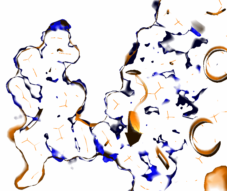
- First, grid points are assigned zeros if they are within a LJ radius (1.2,1.5, and 1,7 Angstrom for H,O/N, and all other atoms respectively) of the nearest protein atom, or a value varying from 0 to 1 if the grid point is within a distance of 2xLJ radii; all other grid points are assigned a value of 1 (see Fig.1).
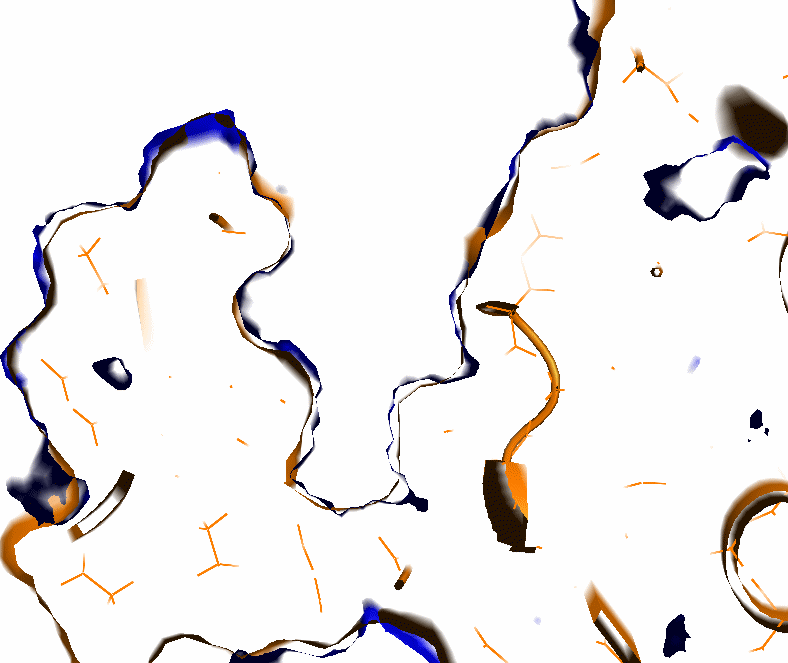
- Small pockets defined by the parameter Averaging (in Å) are eliminated (to speed up calculations at the next step), see input parameter Averaging (see Fig.2).
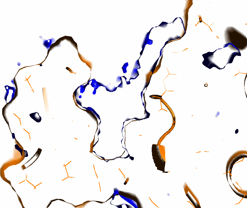
- The protein surface is distinguished from the internal cavities as follows (see Fig.3):
- From each grid point having a non-zero value, a set of vectors with evenly distributed directions is checked (default number of vectors is 12).
- If less than 60% of vectors with a fixed 7 Angstrom length reach protein atoms, this grid point is assigned to the protein surface and is assigned a value of zero, otherwise it is considered as an internal protein cavity.
- This helps to recognize large open cavities and omit small pockets.
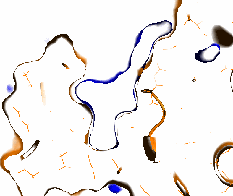
- Pocket boundaries are smoothed by averaging the pocket distribution function within +-1.5 Angstroms of each pocket point. (see Fig.4)