Output of TRAPP-pocket
There are several ways to visualize the TRAPP-pocket results
- You can use Trj-* and/or Combined Trajectories underneath the Identification of transient pockets section of the Trapp Results page. This page of the webserver contains most of the results, including pocket characteristics,
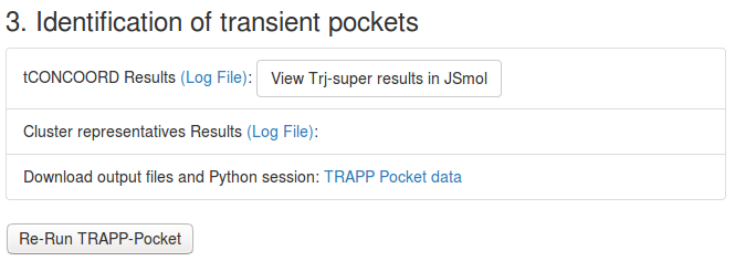
- For more detailed analysis, you can download a compressed archive using the Trapp Pocket data link that includes most of the data generated by TRAPP-pocket and several PyMol scripts for visualization of trajectories and transient/conserved pocket regions .
- Finally, you can visualize the data from the Trapp Pocket data link using another molecular graphics software (for example, VMD or Chimera).
More details of these can be found below:
Pocket Dynamics
Pocket and protein conformations are visualized for each snapshot
(to avoid overloading the computer memory,
the trajectory/ensemble of structures is split into parts of 10 snapshots each)
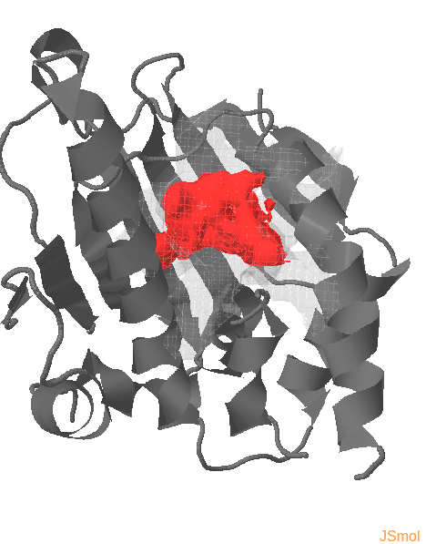
Transient parts of the pocket can be visualized at different occurrences (given in %; see Fig.2):
- Appearing: pocket regions that are not present in the reference structure, but appear in some snapshots of the trajectory/ensemble (shown in red).
- Disappearing: pocket regions that are present in the reference structure, but absent in all snapshots of the trajectory/ensemble (shown in blue).
An averaged pocket distribution is shown in green: the most conserved pocket regions can be seen with an averaged pocket distribution at ~90% occurrence.


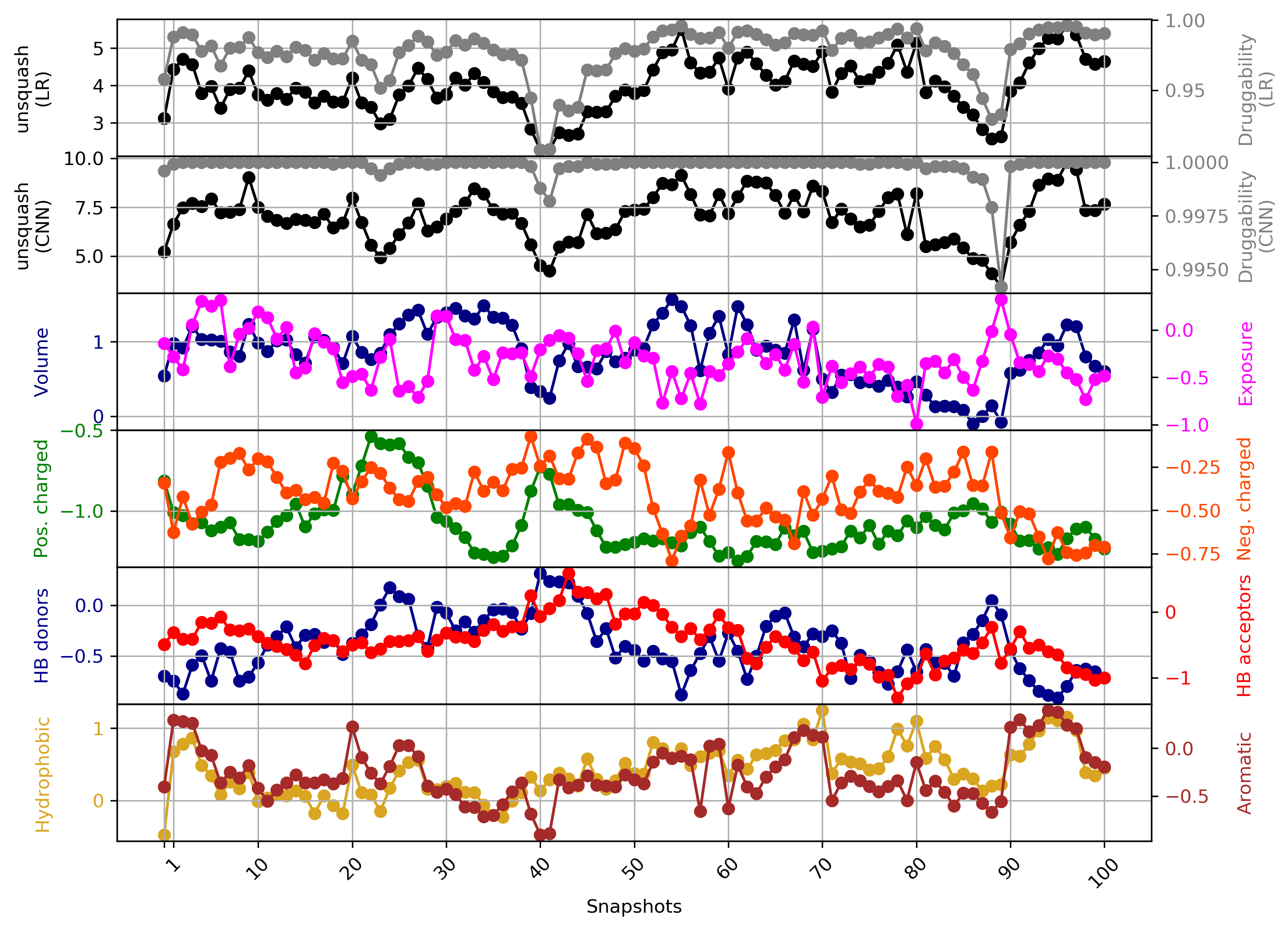
Physicochemical characteristics of the pocket and its and druggability
Variation of binding pocket properties along a trajectory (or along several trajectories) presented:
- Variation of the pocket volume
- The pocket exposure (relation of the solvent-exposed the protein-exposed pocket areas
- Pocket volume around positively/negatively-charged residues, hydrogen donors and acceptors, hydrophobic and aromatic residues
If the druggability computation in the TRAPP-pocket module was selected, additionally druggability generated using logistic regression (LR) and convolution neural network models are shown.
All values are re-scaled and given in the arbitrary units. The link to the original data is given additionally under the plot.
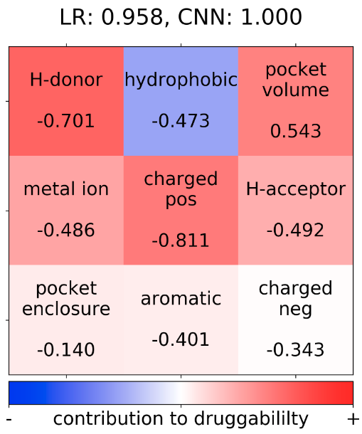
The plot shows a description of the residues involved in the pocket. (Fig.5a) More information regarding the calculation of the residue descriptions and an explanation of the results can be found here.
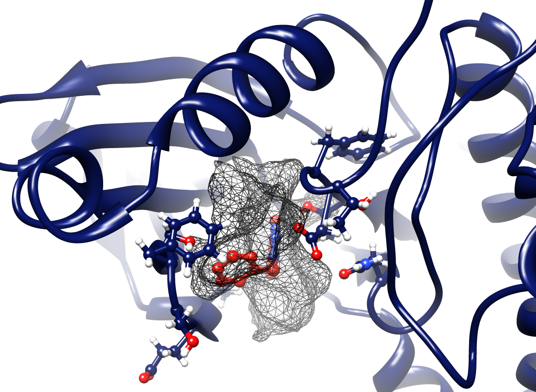
Additionally, for any structure of interest a heatmap for the TRAPP-LR model can be computed (Fig.5b), which shows a contribution of each physicochemical property to the pocket druggability (red- druggable, blue-less druggable); the relative contribution for each property is shown in numbers below each property weight. The pocket regions that mostly contribute to the pocket druggability are visualized in red (Fig.5c)
Pocket contact residues
The set of residues is split into bins; please note, that the residue numbering can differ from the original PDB file: residue number 1 in the figures is the first residue in the reference file.
- For a particular trajectory (Fig.6):
Color defines the number of heavy atoms in each residue that contribute to the pocket boundary in a particular snapshot.
The last line in each bin (denoted by "0") shows the number of heavy atoms in each residue that contact a pocket in the reference structure.
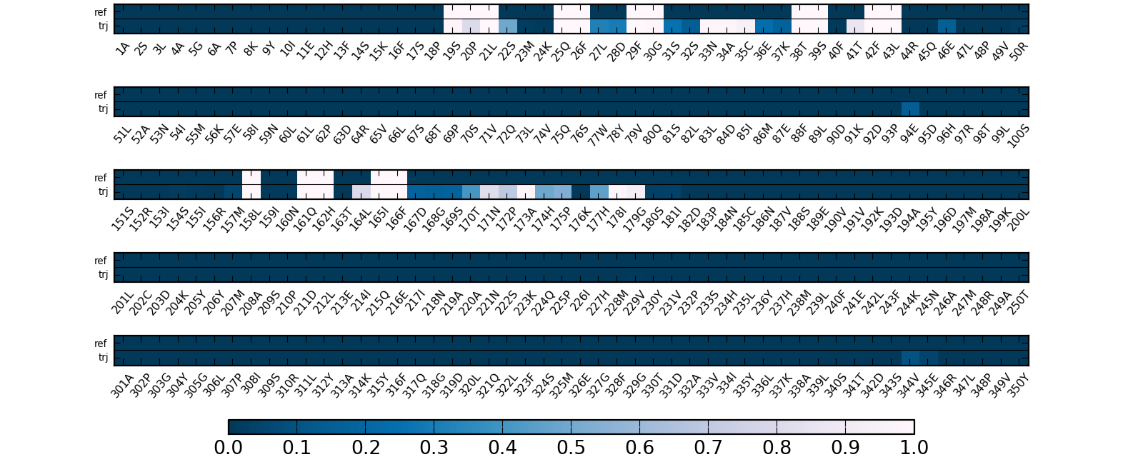
- Summary over all trajectories (Fig.7):
The upper line shows residues that contribute to the pocket boundary in the reference structure.
The lower line in each bin of the plot contains the fraction of snapshots in which a particular residue has contacts with the pocket.

Show transient sub-pockets and their characteristics
Choose a transient pocket occurence (in %) at which you would like to split the transient pockets into transient regions/sub-pockets and to analyse each region/sub-pocket separately (a new window will be opened).
The transient region is split into sub-regions (sub-pockets) and the degree of their opening is computed for each snapshot/structure in a trajectory or within an ensemble.
Visualization using PyMol sessions
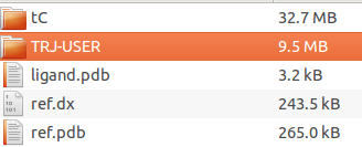
The archive that can be downloaded by clicking on the Trapp Pocket data link contains a PyMol folder, which contains the following data:
- Ligand PDB structure (ligand.pdb)
- Reference PDB structure (ref.pdb)
- Pocket of the reference structure in dx format (ref.dx, can be visualized with VMD, Chimera, or PyMol software)
- Directories with data generated by each method separately (tCONCOORD, L-RIP, RIPlig, or MD) or/and trajectory uploaded (named TRJ-USER), which contains transient (tranisent.dx) and conserved pocket regions, (conserved.dx)
- PyMol directory with PyMol scripts for visualization of results:
- Scripts that summarize results for each trajectory separately
- For each snapshot, a grid is loaded in a separate group: snap_1, snap_2 etc....
- Additionally, at the end of the snapshot list, the following files are loaded :
- Transient and conserved regions of a particular trajectory are shown by red/blue and gray mesh, respectively.
- The binding pocket in the reference structure is shown by a green surface refpock.
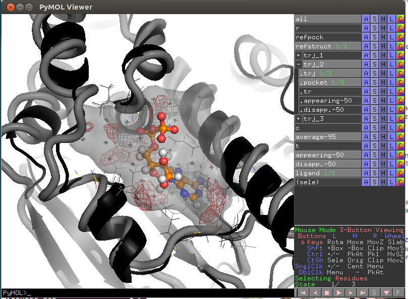
- Script PyMol/lj_trajectories.pml.pse
- refstruct (black cartoon) - reference structure, active site residues are shown by lines;
- refpock - a reference pocket;
- Transient pocket regions appearing-50/appearing-25 and disappearing-50/disappearing-25 are shown by red/blue meshes (that appear/disappear in 50%/25% of snapshots relative to the pocket in the reference structure);
- average-95- most conserved pocket regions (exist in 95% of all snapshots);
- appearing-50/25 and disapp.-50/25 - transient pocket regions that appear/disappear in 50%/25% of snapshots relative to the pocket of the reference structure
Files PyMol/grids-trj_1.pml, PyMol/grids-trj_2.pml, etc. are generated for each protein trajectory and contain the pocket representation (using a corresponding grid file snap.*.dx) and protein structure for each snapshot as well as conserved and transient regions for this particular trajectory separately.
Each group includes a protein structure (.s* - shown by gray cartoon if selected) and a pocket shape (.pocket* - shown by gray isosurface)
-the reference structure (refstruct, shown by black cartoon with the active site residues shown by lines), the reference binding pocket (refpock).
-the ligand structure used for identification of the binding site (ligand.)
Appearing-50/disapp-50 and appearing-25/disapp-25 show transient pocket regions that appear or disappear in at least 50% or 25% of snapshots, respectively.
Averaged - pocket regions that are present in all snapshots are shown in gray mesh.
File lj_trajectories.pml summarizes all pocket motion trajectories in "pseudo-atom" representation. It also contains conserved and transient regions identified from all trajectories and from each trajectory separately.
Each group trj_1, trj_2 etc. contains a particular motion trajectory of a protein ("trj") and a binding pocket ("pock")
The pocket is represented by pseudo-atoms. (See. Fig.13-16)
Note that pseudo-atoms reproduce the pocket shape rather roughly. For a more accurate representation, use the grid view (script grid-trj_*.pml);


Understanding the output data
The general structure of files generated by TRAPP
Complete list of output files
By clicking on the Trapp Pocket data link, you can view many different input and output files. The organisation and content of these files depends on the input files, parameters and methods that are used.
| File name/PATH | Content | Comments |
|---|---|---|
| contact_residues_ref.dat | residues that define a binding site and are used for superimposition of structures and building of a pocket grid | chosen on the basis of the input parameters : ligand or binding pocket center and radius. |
| contact_residues_ref.pdb | residues that define a binding site in PDB format | - |
| conserved.dx | conserved pocket regions that appear in each snapshot of each trajectory | - |
| ref.pdb | reference structure | ref.structure from the input file, but with checked or changed atomic names, added H etc... |
| ref.dx | reference binding pocket | binding pocket of the structure "ref.pdb" ; in dx ASCII format |
| transient.dx | transient pocket regions averaged over all snapshots/trajectories | - |
| TRJ1/trj_1.pdb | a particular trajectory used for analysis | atom names changed for GROMACS, with hydrogen added, and superimposed |
| TRJ1/LJ-OUT/lj-pocket_trj_1.pdb | pocket motion trajectory for a particular protein trajectory 1 | a protein cavity is represented by a set of pseudo- atoms (radius is defined by the input parameter) that fills a pocket grid at a particular ISO-value ; cavity snapshots for each protein motion trajectory are concatenated into a pocket trajectory |
| TRJ1/LJ-OUT/pca-eval-trans.*.dat | PCA eigenvalue computed from the pocket variations over all snapshots for a particular trajectory 1 | see input parameters of the PCA procedure |
| TRJ1/LJ-OUT/snap.*.dx | position and shape of the binding pocket for each snapshot of a particular trajectory. | The grid values are varied from 0 (inside a protein body or in a protein exterior region) up to 1 in the pocket region. - Isopotential surface at a value of about 0.6 corresponds to the van der Waals surface of a protein. |
| TRJ1/LJ-OUT/averT_1.dx | averaged binding pockets over all snapshots of a particular trajectory 1 | - |
| TRJ1/LJ-OUT/transT_1.dx | transient pockets regions averaged over all snapshots of a particular trajectory 1 | - |
| PyMol/lj_trajectories.pml | PyMol script for overview of TRAPP output | - |
| PyMol/grids-trj_*.pml | PyMol script for visualization and analysis of TRAPP output for each snapshot in a particular trajectory | - |
| JMOL/models/TRJ1/jmol.html | JSmol script for overview of TRAPP output | for a long trajectory only 200 snapshots (selected at equal intervals) are shown |
Visualization of the pocket using molecular graphics programs
*.dx grid files and can be visualized in different molecular graphics programs (VMD, Chimera).