TRAPP input parameters
General input parameters and commands
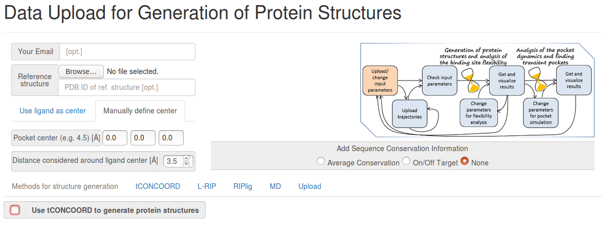
- PDB structure: A protein structure that will be used as a reference (for alignment of trajectories, generation of protein conformations, and also for identification of transient pocket regions).
- PDB ligand file: The position of the binding pocket will be defined by the corresponding ligand taken from the co-crystallized structure.
- Manually defined pocket center in Å (x y z): The position of the binding pocket will be defined using coordinates of the pocket center (defined with reference to the coordinates of the reference protein structure).
- Distance considered around ligand center: The distance (in Å) from the centres of ligand atoms (or the binding pocket center) that is used to identify putative binding site residues. These binding site residues are then used for alignment and superimposition of the protein structures.
Sequence Conservation Information
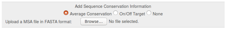
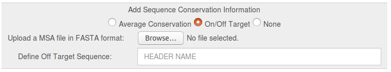
This option can be used to upload a multiple sequence alignment (MSA) in FASTA format and calculate a conservation score, which is then visualized on the reference structure together with the TRAPP pocket results. See the documentation page for more details.
- None: This is the default setting which means that no sequence information is taken into account
- Average Conservation: Calculation of the average sequence conservation of the uploaded MSA and visualization on the reference structure in the final TRAPP Pocket results. See Fig.2a
- On/Off Target: Calculation of the difference in the sequence conservation of the uploaded MSA (Off and On Targets) and the MSA without the Off target sequence. The Off target sequence has to be identified by the Header name in the MSA file. The difference is visualized on the reference structure in the final TRAPP Pocket results. See Fig.2b
Parameters for TRAPP-structure
Method(s) to be used for generation of protein structures: You can choose a method (then TRAPP-structure and TRAPP-analysis will be performed) or upload already available trajectories (then only TRAPP-analysis will be performed).
tCONCOORD Advanced Settings:
- Ensemble: For tCONCOORD, the size of the ensemble of structures must be defined.
- Minimize generated structure: Each tCONCOORD structure will be minimized using NAMD.
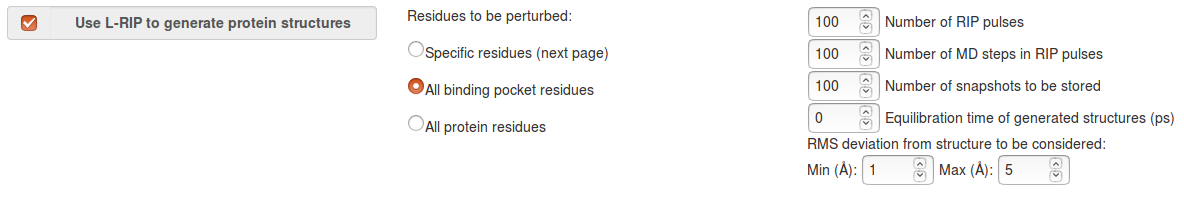
L-RIP Advanced Settings:
- Residues to be perturbed: You can choose either:
- Perturb specific residues (numbering starts from the first residue in the reference structure)
- Each residue of a binding site
- Each residue in a protein (this is not recommended since it may take a lot of computation time).
RIPlig Advanced Settings:
- Phe or Leu: An artificial ligand can be chosen. An artificial ligand is just a residue (Phe or Leu) with a capped backbone. It will be placed in different parts of the binding pocket and perturbed using the RIPlig approach.
- Place pseudo-ligands in neighbor cavities: You can choose whether the pseudo-ligand will be placed only in the central binding pocket (as defined by a ligand or pocket-center position) or also in other cavities if they are present around the central binding pocket. In the latter case, more flexible elements can be found, but a longer simulation time is required (a larger number of trajectories is generated).
- Limit the number of trajectories to be generated by: The number of trajectories to be generated may be limited (useful for test running). The number of trajectories generated by RIPlig corresponds to the number of different positions of the pseudo-ligand in the binding pocket.
- Seed number for generation of pseudo-ligand position: If 0, positions will be generated randomly; if a non-zero number is given, RIPlig simulations can be reproduced. This can be used, for example, for running additional MD equilibration on RIPlig trajectories already generated (trajectories generated once will not be re-generated in the same session).
L-RIP & RIPlig Joint Parameters:
- Number of L-RIP pulses: Default value: 100. The value must be less than 300; more pulses generate larger perturbations. The length of the trajectory increases linearly with the number of pulses.
- Number of MD steps in L-RIP pulses: The length of the implicit solvent MD run that is applied after each perturbation step of each time step is 0.002ps. This value must be in the range 100-300 steps i.e. The MD run is 0.2-0.6ps in duration. Longer equilibration takes more time but helps to localize perturbation around perturbed residues and to reduce protein heating, therefore making it possible to increase the number of pulses without the protein overheating, which improves sampling of the conformations of flexible elements.
- Number of snapshots to be stored: Each trajectory generated by L-RIP/RIPlig consists of snapshots (the default value is 100 corresponding to the Number of L-RIP pulses). You can choose to store only some of the snapshots and use them for further analysis.
- RMS deviation from structure to be considered: Only conformations that have RMSD (in Å) from the reference structure within the given limits will be stored. This helps eliminate conformations that are close to the original (reference) structure as well as conformations that correspond to extremely large distortions of a protein.
- Equilibration of generated structures: The length of equilibrium in ps for L-RIP/RIPlig conformations will be equilibrated using implicit solvent MD and the final snapshot will be used for further analysis and pocket simulations.
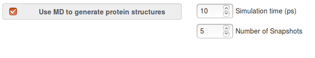
MD Advanced Settings:
- Simulation time: For implicit solvent MD, a simulation time in ps must be defined: the simulation timestep in MD is 0.002 ps. (Langevine dynamics and the SASA model are used).
- Number of snapshots: For implicit solvent MD, the number of snapshots to be stored must be defined.


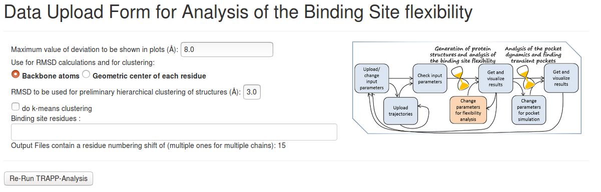
Parameter for TRAPP-analysis
- Maximum value of deviation to be shown in plots: Threshold value of RMSD (in Å) for each binding site residue from those of a reference structure to be shown in plots
- Backbone atoms or Geometric center of each residue: The RMSD of the backbone atoms or of the position of the geometric center of the binding site residues is to be used for comparison with the reference structure and for clustering.
- RMSD to be used for preliminary hierarchical clustering of structures: A maximum RMSD value (in Å)(of either the backbone atoms or the geometric center of all heavy-atoms) for any residue of the binding site is used for clustering.
- Do k-means clustering: If not checked, only preliminary single-linkage hierarchical clustering is carried out. It is much faster, but only gives a rough idea of how diverse the binding site conformations are (each structure is compared against the first element of the cluster only, as this reduces the computing time). Otherwise, k-means clustering will be performed, and this may take much more computational time. The number of clusters that is used, is taken from the preliminary clustering.
- Binding site residues: Changes the binding site residues that will be used for alignment and clustering of structures and visualisation of results.
Parameters for TRAPP-pocket
Structures to be used for identification of transient pockets:
- Trajectories: You can choose either all of the generated or uploaded ensembles of structures to be used for binding pocket simulations or only some of them.
- Cluster Representatives: Results of the last TRAPP-Analysis step (if k-means option was selected, this is the representatives of k-means clustering)
- H-atoms to be generated for the reference structure and/or H-atoms to be generated for structures in trajectories: H-atoms can be generated (using NAMD) for a reference structure or for all snapshots of a trajectory or ensemble of structures. This is useful if crystal structures are used for TRAPP-pocket analysis.
Analysis of transient pocket regions:
- Analysis will be done of the pocket occurrence of (%): Used for visualization of transient regions in JSmol. Several values can be specified. Note, that each additional value notably increases computational time. Choose 10-20% for a pilot run.
- Run PCA: Principle component analysis of the variation of the pocket distribution function along a trajectory or within an ensemble. This procedure is extremely time - and memory- consuming. If the PCA matrix is too large for the available RAM, the program can crash. Moreover, the 3D distribution of the PCA vectors may become extremely complicated. Thus, it is strongly recommended to run PCA only if several structures are analyzed.
- Run clustering: Used to split transient regions into sub-regions (transient regions are selected at a certain given occurrence(see above)). The sub-regions (or sub-pockets) are visualized in JSmol. Besides this, the opening of these sub-regions will be traced along the trajectory, which makes it possible to find snapshots (structures) where a particular sub-region is mostly open or closed. Additionally, statistics of the sub-region opening will be provided.
Define pocket position and grid size:
- Use TRAPP-analysis based binding site residues: You can also re-define the binding site to be used for pocket analysis, by giving explicitly the residue number (remember, that the internal residue numbering is changed - the numbering starts from 1 in the reference structure).
- Use distance around the considered ligand: Used for the binding site definition (it may be different from that used for structure generation and for TRAPP-analysis).
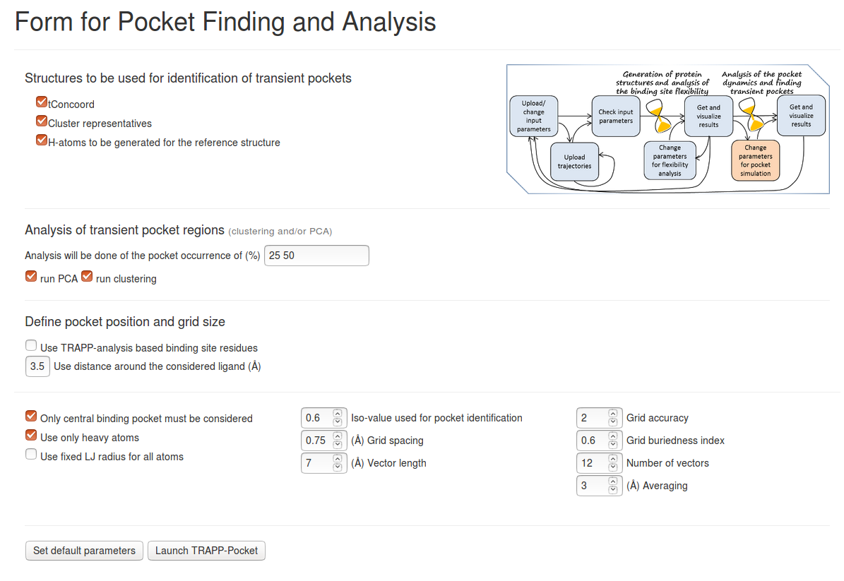
Advanced parameters for the pocket identification procedure:
- Only central binding pocket must be considered: Defines whether all cavities or only the central binding pocket must be used for analysis (default: yes; each cavity that is connected with the central pocket in at least one snapshot will be considered). The position of the central pocket is defined by the ligand or pocket center (as provided by the user); all cavities that directly contact the central pocket are assigned to the central pocket. If only central binding pocket must be considered is switched off, all small cavities that never directly contact the binding pocket defined by the user will also be traced and analyzed.
- Use only heavy atoms: If checked, a Lennard Jones radius of 1.8 Angstroms is used to take into account the presence of H-atoms. The Lennard-Jones radius can also be modified (see Fixed LJ radius for all atoms to be used), otherwise atom-type dependent Lennard-Jones radii will be used.
- Fixed LJ radius for all atoms to be used: If checked, for pocket simulations a single value of the Lennard Jones radius will be used (otherwise it is 1.2, 1.5, and 1.7 Angstroms for H, O/N , and all other types of atoms)
- Iso-value used for pocket identification: The value of the cavity distribution function to be used for pocket definition (default: 0.6 , that corresponds approximately to a van der Waals surface of a protein)
- Grid spacing: Used for pocket simulation. It is strongly recommended to use the default value which is less than the average Lennard-Jones radius of atoms (the default value is 0.75 Angstroms). However, computational time increases as the grid size increases.
- Vector length: The distance used to estimate the extent to which a particular grid point is buried (default: 7 ). This parameter is used to distinguish between protein cavities and protein surface.
- Grid accuracy: Defines accuracy of the simulation of pocket buriedness (1 or 2, default: 2 ). The value 2 means that each grid point will be probed for whether it belongs to the pocket or to the outside of the protein twice: using vector length = Vector length/2.0 and Vector length.
- Grid buriedness index: Coefficient (from 0.0 to 1.0) that defines the degree of buriedness of a pocket point (default: 0.6 ). The parameter is used to distinguish between protein cavities and protein surface
- Number of vectors: Defines the number of vectors that will be used for distinguishing between protein interior and exterior regions (default: 12 )
- Averaging: Used to eliminate small cavities (those that cannot fit at least one ligand atom) and to smooth the pocket boundary (default- 3 Angstroms )
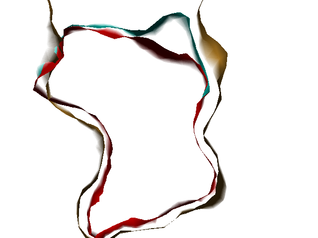
Example illustrations for identification of the pocket shape
- Vector length: If the value is small, large and open pockets will not be recognized. If the value is large, shallow cavities at the protein surface will be identified as pockets. Small pockets are better recognized at smaller vector lengths.
These example images show some of the possible outputs when changing the input parameters associated with the pocket shape. These parameters can be set when clicking on Run Trapp-Pocket. Different molecular graphics programs can then be used to visualise the results.
- Number of vectors: Smaller values decrease the quality of the pocket definiton, but increase the speed. At low accuracy, some small pockets may be missing and the boundary between the pocket and protein exterior may not be accurate.
- Grid accuracy: For example, the combination of vector length = 7.0 and grid accuracy = 2 means that at first a vector length of 3.5 Angstroms will be used, and then, if the current grid point has no protein contact percentages above the threshold of the grid buriedness index, the vector length of 7.0 Angstroms will be checked; if grid accuracy = 1 is used, only the vector length of 7 Angstroms is used.
The boundary between a pocket and the protein exterior volume becomes smoother as the number of directions increases.
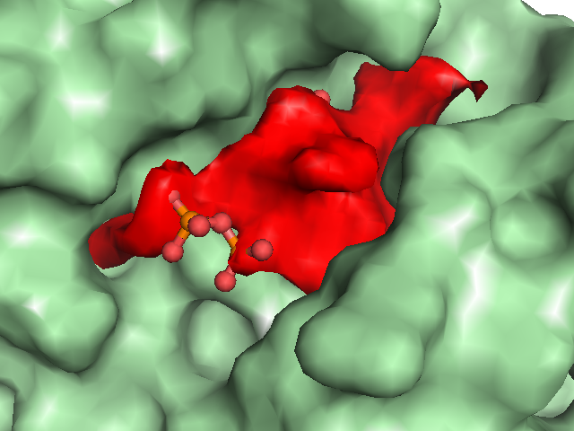


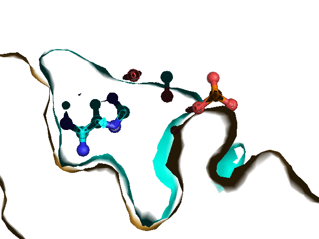
- Grid buriedness index: Use small values (0.5-0.6) to find large open pockets or shallow pockets on the protein surface.