Exploring cryptic pocket formation in MD trajectories generated by L-RIP
In this example, a MD trajectory generated by L-RIP is used for identification of cryptic binding pockets in p38 MAP kinase
1. Overview:
In early stages of drug discovery, accurate protein druggability prediction is essential for lead molecule selection. Although, accurate pocket druggability is difficult to predict when the transient changes in binding pocket due to conformational changes gets taken into consideration. The analysis of binding pocket variations is difficult with the traditional structural determination methods such as X-ray crystallography and NMR as these techniques struggle to capture all possible conformations of the protein in order to get the accurate picture of pocket mobility.
Here, we analyze the pocket druggability using trajectories generated from a molecular dynamics simulation to identify potentially druggabile conformation in p38 MAP kinase.
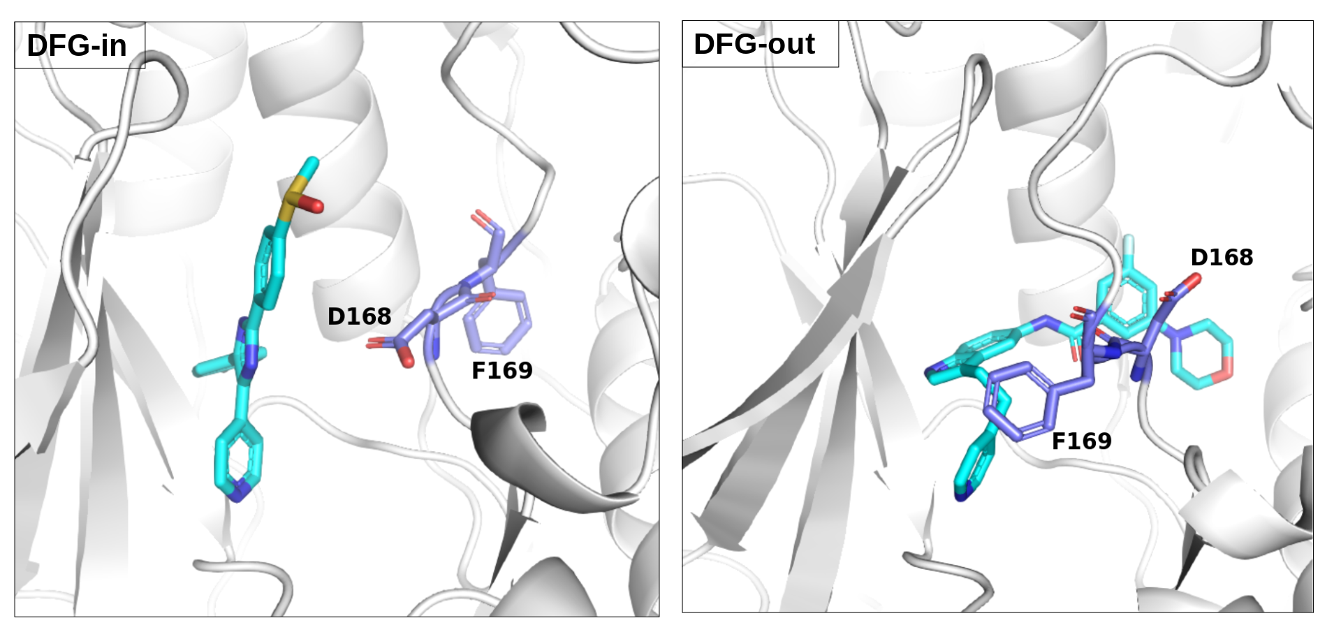
There is an ATP-binding pocket that forms in between a flexible beta-sheet and two flexible loops - one of them being a DFG loop (highly conserved Asp-Phe-Gly motif). Within this loop, phenylalanine at position 169 shifts between its buried position (DFG-in conformation) and an out-ward position (DFG-out conformation) that interferes with ATP-biding. DFG-out conformation also results in the opening of a hydrophobic cryptic pocket adjacent to the ATP binding site. As there are inhibitors that exploit this cryptic pocket, the pocket druggability differs between the two conformations. DFG-in conformation is seen in crystal structure 1a9u and DFG-out in the crystal structure 1wbs.
Example from Jui-Hung Yuan, et al - submitted to JCIM
2. To run these examples, you need the following files and parameters:
- prot.pdb The reference structure (generated from the 1r3c pdb file)
- ligand.pdb The ligand that will be used for defining the binding site.
- trj_LRIP_snaps_1_100.pdb MD trajectories generated using L-RIP, with 300 perturbation pules and 300 implicit solvent MD steps after each pertubation (first 100 snapshots used).
We use default value for pocket radius = 6.0 Angstroms. (The druggability result might be affected when different pocket radius is used.)
3. Simulation procedure and results
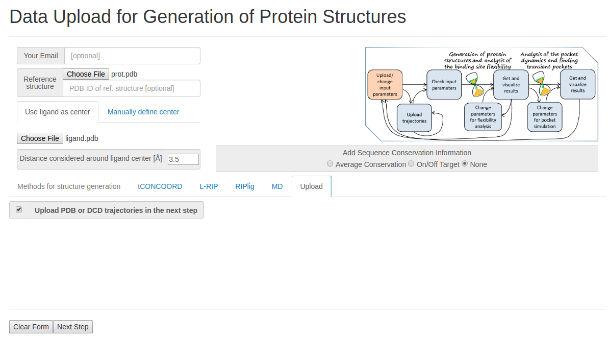
- Step 1: Uploading reference structure and defining input parameters
You have to upload the reference structures of the protein and ligand and click Upload trajectories at the next step before you go to the Next Step.
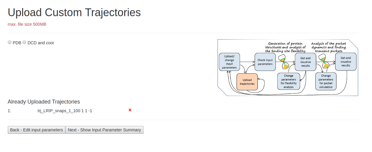
- Step 2: Uploading Trajectories
On the page Upload Custom Trajectories, you can upload desired PDB trajectory file. Check if correct PDB file is uploaded at the bottom of the page. Then click Next page to proceed.
- Step 3 : Checking input data and starting simulations
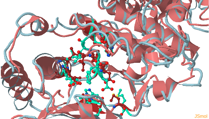
This page shows the JSmol visualization of the reference structure and an identified binding pocket. Click Launch TRAPP-structure/analysis to start the analysis. Since no method for generation of new structures was selected in the previous step, only analysis of the uploaded structures (trajectories) will be done.

- Step 4: Viewing simulation results of TRAPP-analysis
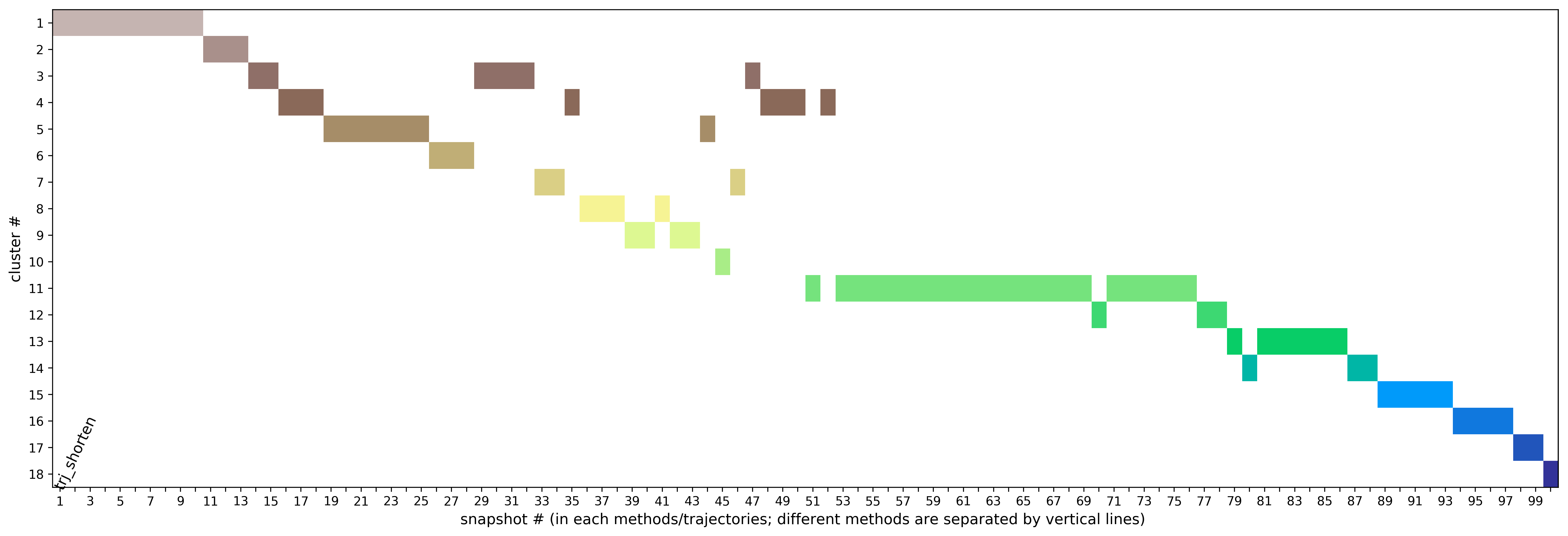
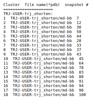
Preliminary results are available in the link View Analysis. Note that TRAPP-analysis runs with default parameters (backbone atoms used for RMSD calculations and a fast hierarchical clustering of the binding site conformations carried out with a threshold of 3 Angstroms). include residues that are not related to the binding site regions (use the link View cluster representatives in JSmol for a view of selected binding site residues that are shown by sticks). This can be corrected by changing parameters and clicking re-run TRAPP-analysis.
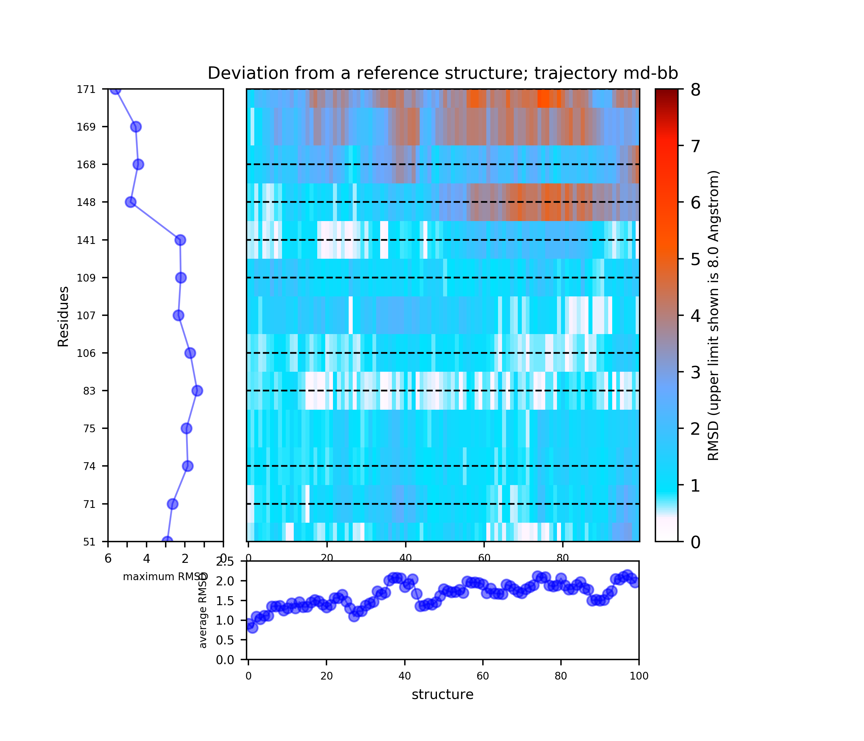
Binding site motions were found around residues 168-169 DFG and part of the activation loop).
- Step 5: Editing TRAPP-pocket parameters and running TRAPP-pocket
- Check Use TRAPP-analysis based binding site residues: To make sure that all binding site residues are included in pocket simulations.
- Check H-atoms to be generated for the reference structure but uncheck H-atoms to be generated for structures in trajectories since the trajectories are not from an original structure.
- Check run PCA and run Clustering.
- Check Calculate Druggability to make druggability prediction by applying the grid settings from the TRAPP-LR/CNN models that are trained on the bindability datasets.
- Launch TRAPP-pocket.
For our example the Trapp-pocket parameters are adjusted as follows:
- Step 6: Understanding TRAPP-pocket results
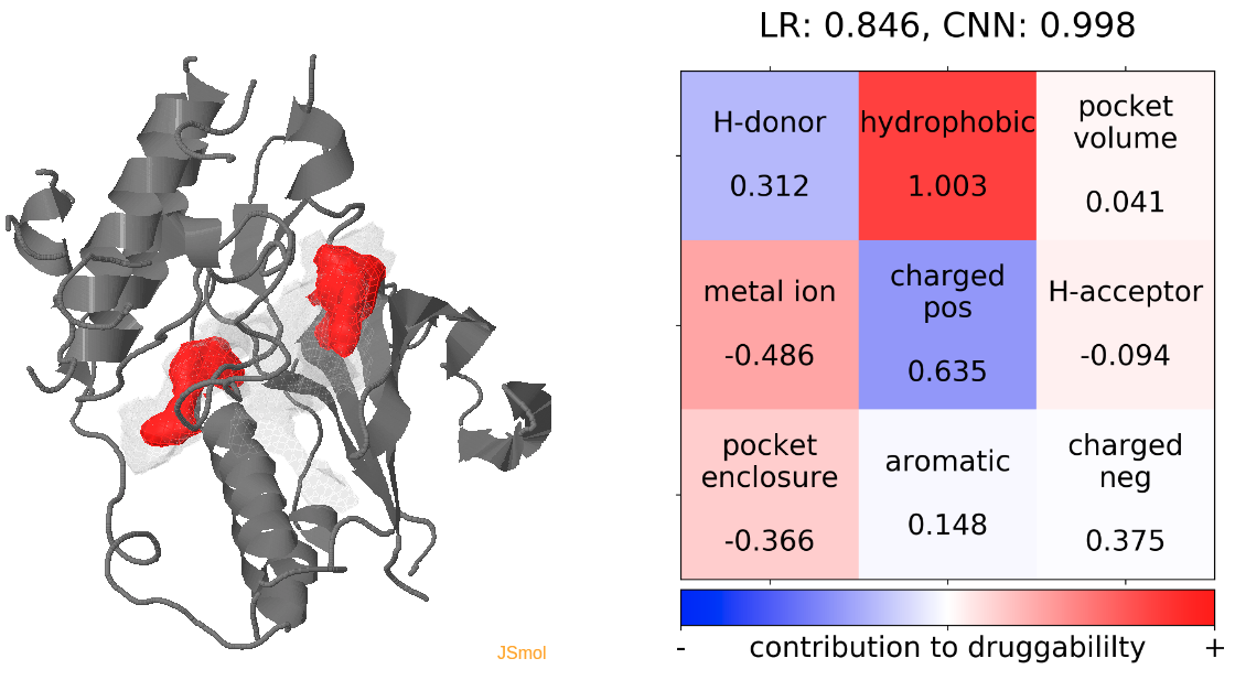
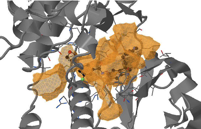
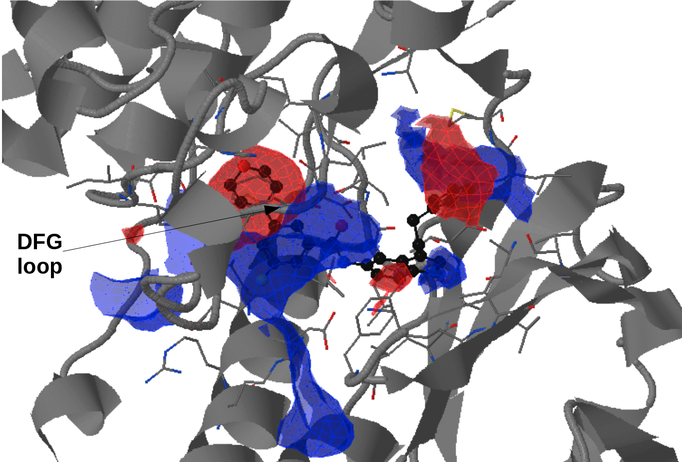
- Under Change JSmol View tab, the pocket from the reference strucutre (yellow) is displayed along with the reference structure. The appearing (red) and disappearing (blue) pocket regions from the trajectories can be displayed by selecting the respective occurance percentage. (See Fig.14, Fig.15)
- The motion of DFG loop can be observed from the pocket regions appearing and disappearing around the cryptic pocket. (Fig.15)
The TRAPP-pocket simulation results for the uploaded trajectory can be viewed using the link: View Trj-trj_LRIP_snaps_1_100 results in JSmol results in JSmol that uses JSmol for visualization of transient pockets:
- Step 7: Analyzing TRAPP-pocket druggability results
- Snapshot 0 refers to the pocket druggability data obtained from the reference structure. (See Fig.12)
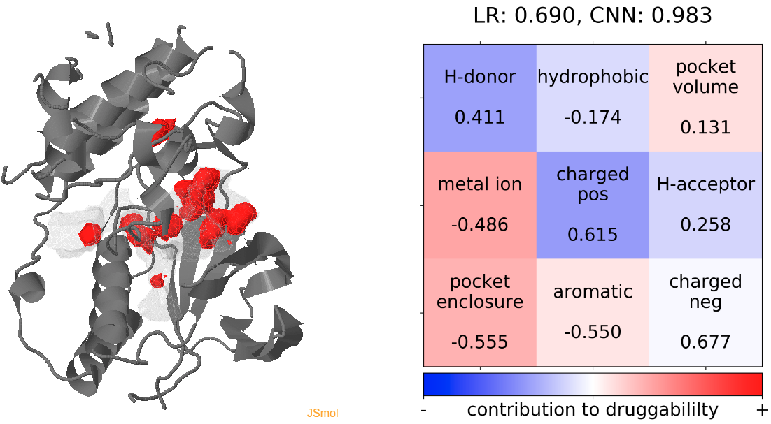
- The point with the lowest druggability score in the MD trajectory is at snapshot 7, where the connection to the sub-pocket is blocked by the H-bonding between D168 and K53. In alignment with this result, the low druggability seems to be mainly caused by the presence of H-donor and positively charged residues inside the binding pocket. (See Fig.13)
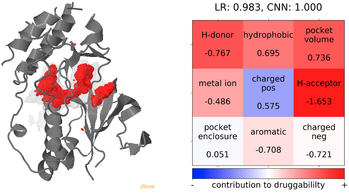
- The highest druggability score is at snapshot 81, where the DFG-out conformation is achieved. The absence of H-bond donor and acceptor, pocket volume and hydrophobility are the major contributors to druggability. (See Fig.14)
The results of TRAPP-pocket druggability are available under the Pocket characteristic tab.
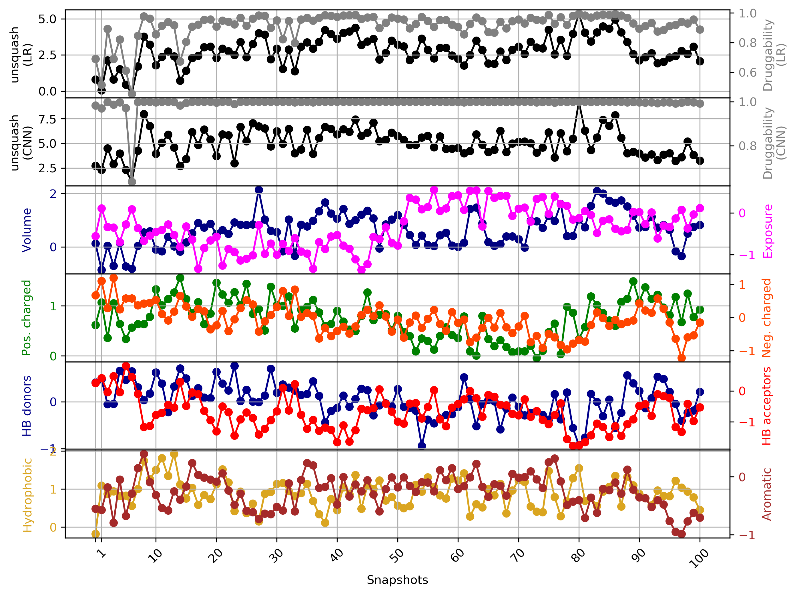
Click Pocket characteristics and druggability to visualize different physicochemical characteristics of the pocket and their contribution to the druggability (See Fig.11).
The druggability score of each frame in the MD trajectory was predicted by both TRAPP-LR and TRAPP-CNN models. The pocket druggability at a specific point in the MD trajectory can be analyzed by choosing the respective snapshot and clicking Load Result in Druggability information for selected snapshot section.