Simulation of binding pocket flexibilty
In this example, L-RIP and RIPlig simulations of HSP90 will be analysed.
1. Overview:
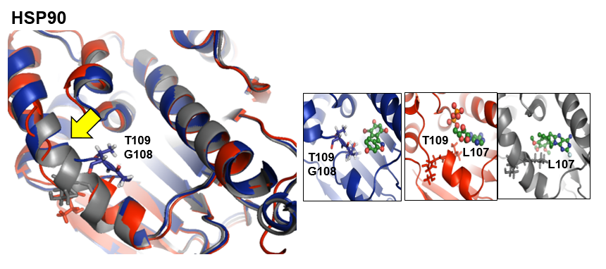
The heat-shock protein HSP90 is a potential target for the treatment of cancer by inhibition of its ATPase activity. The ADP binding pocket contacts an unstable alpha-helix that undergoes distortion in the middle, converting into two short helices connected by a loop inbetween. (PDB structure: 1UYD ; Reference ligand: ADP)
In this example, two sets of trajectories are simulated by using the L-RIP and RIPlig methods. These methods can be done simultaneously (as shown in this example) or separately. Then the simulated trajectories are analyzed using TRAPP-analysis and TRAPP-pocket.
2. To run these examples, you need the following files and parameters:
- 1UYD_protein.pdb
- 1UYD_ligand.pdb
Protein PDB structure (extracted by "grep ATOM 1UYD.pdb > 1UYD_protein.pdb" from the co-crystallized structure)
Ligand PDB structure (extracted by "grep HET 1UYD.pdb > 1UYD_tmp.pdb; grep -v HOH > 1UYD_ligand.pdb" from the same structure)
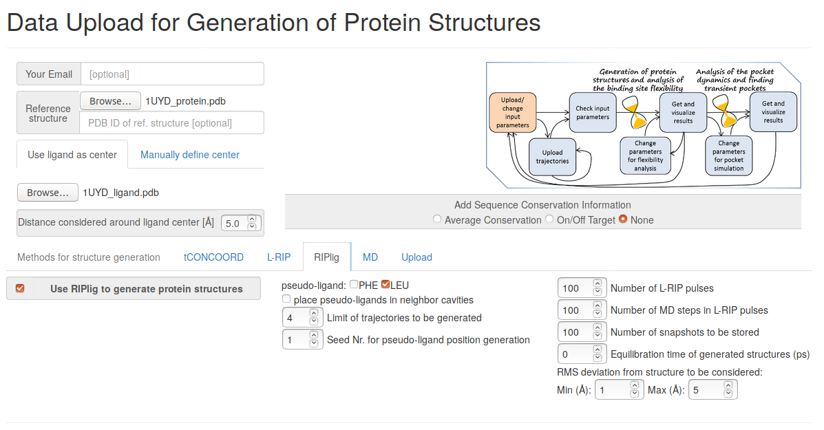
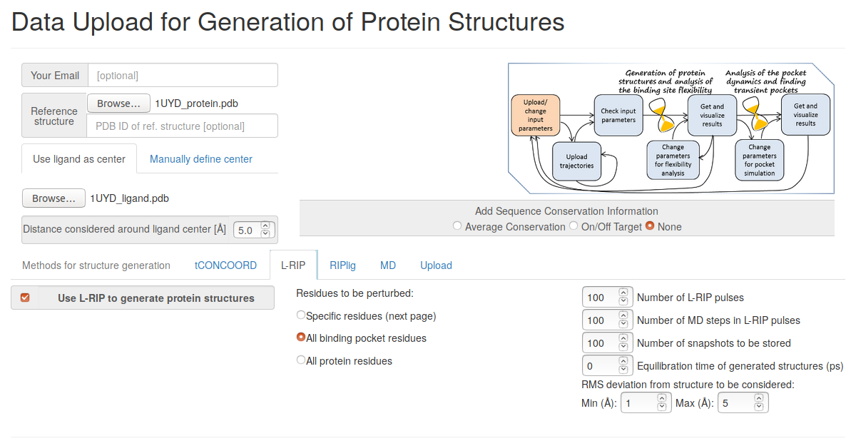
- Step 1: Uploading input data
Upload the reference protein and ligand structures (1UYD_protein.pdb and 1UYD_ligand.pdb), set the radius around the ligand center to 5 Angstroms, choose RIPlig methods for simulation, give the number of RIPlig snapshots to be stored (100 is chosen in the present example).
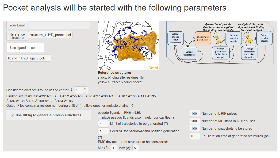
- Step 2:Preview and Starting simulations
On the next page Pocket analysis will be started with the following parameters you must be able to see the JSmol visualization of the reference structure, a ligand, as well as identification of the binding pocket.
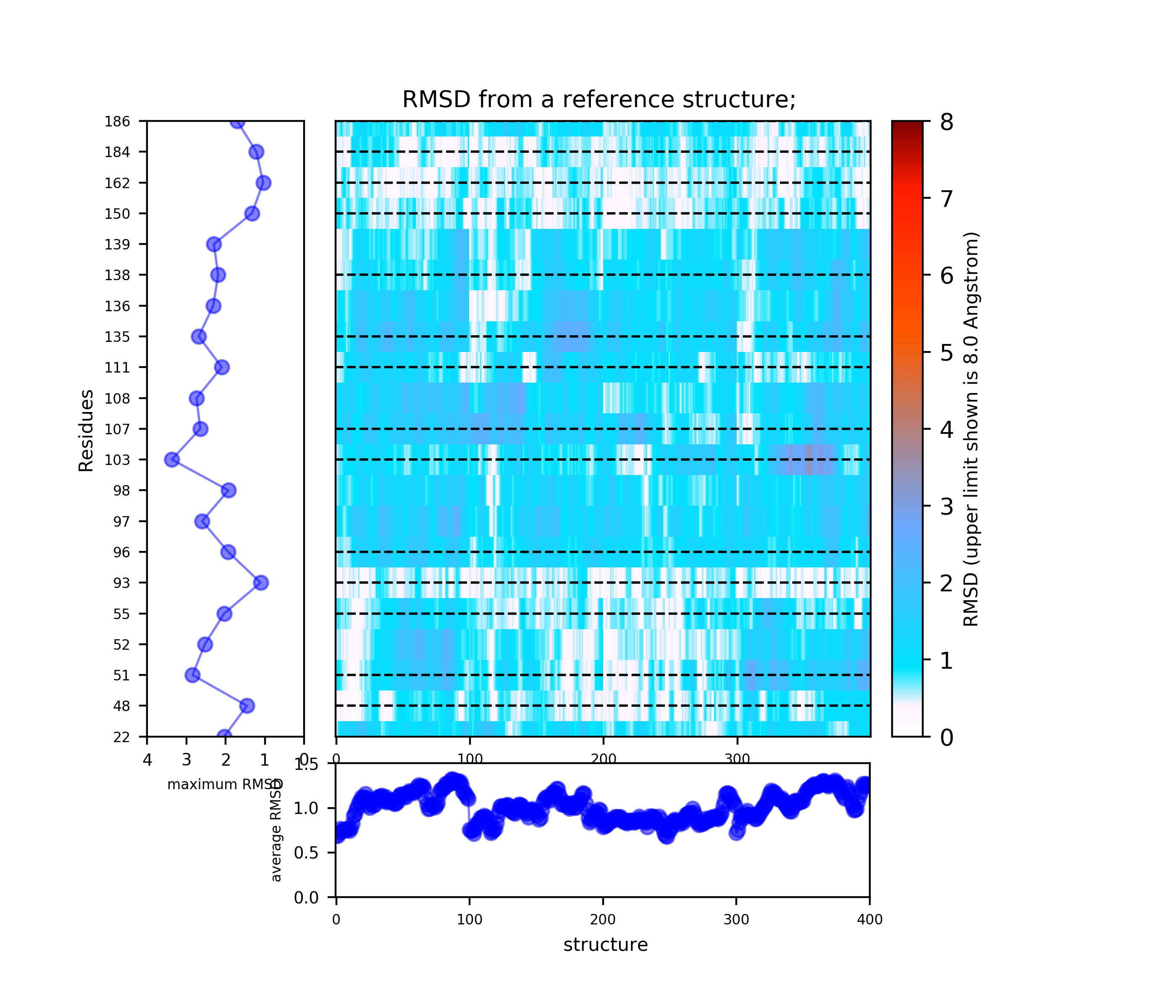
- Step 3: View results of TRAPP-structure and TRAPP-analysis
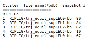
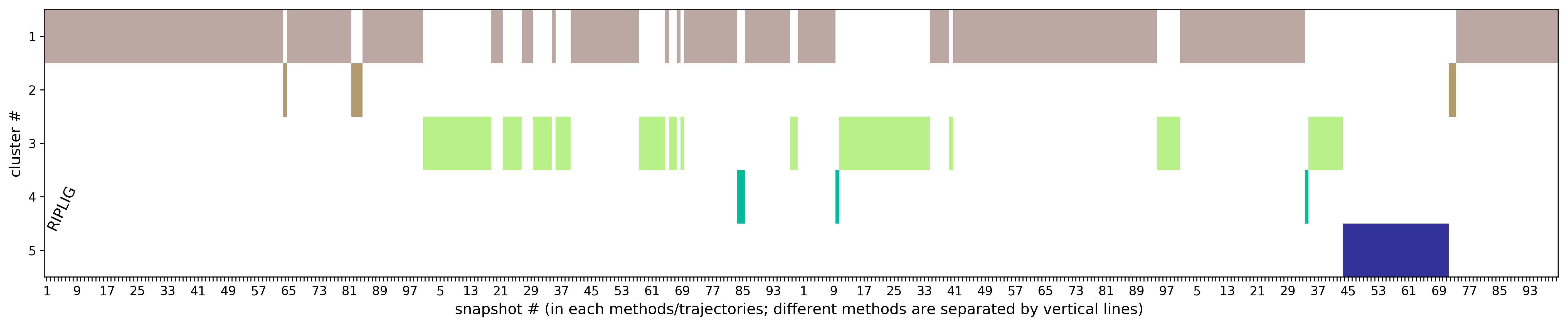
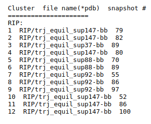
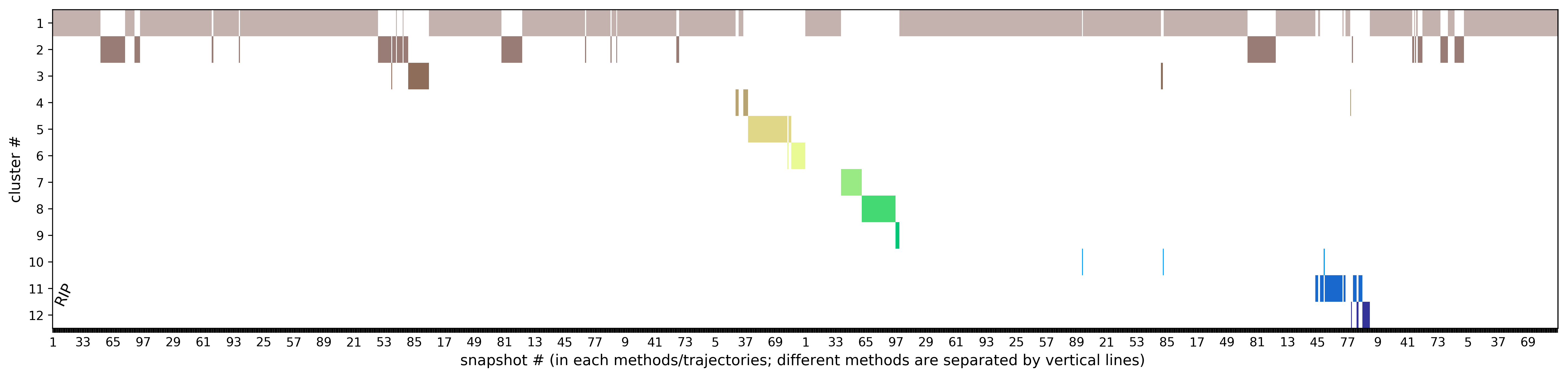
Use the link View Analysis and View cluster representatives in JSmol
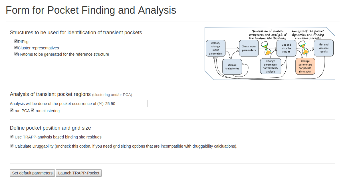
- Step 4: Run TRAPP-pocket
Click run PCA and run Clustering. Analysis will be done at the pocket occurrence of (%) of 25, 50. Check the Calculate Druggability box to compute pocket druggability. Click Launch TRAPP-pocket to start.
- Step 5: Understanding TRAPP-pocket results
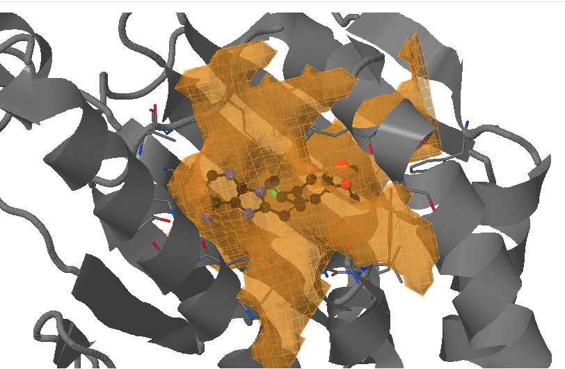
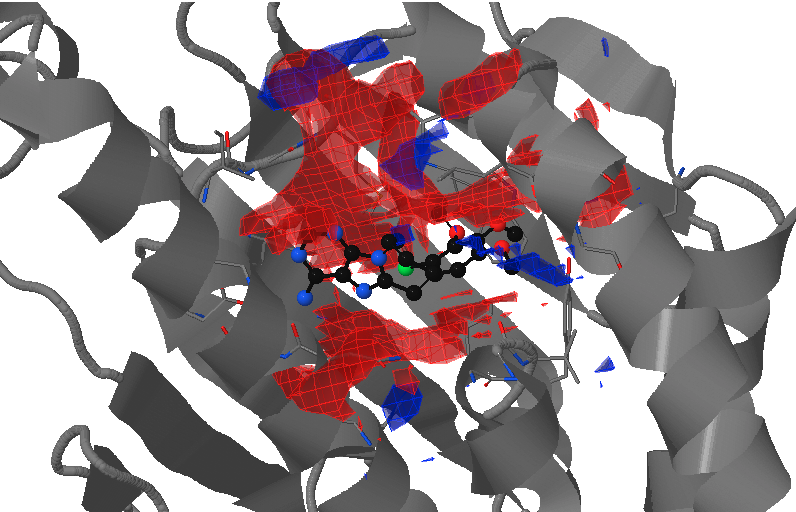
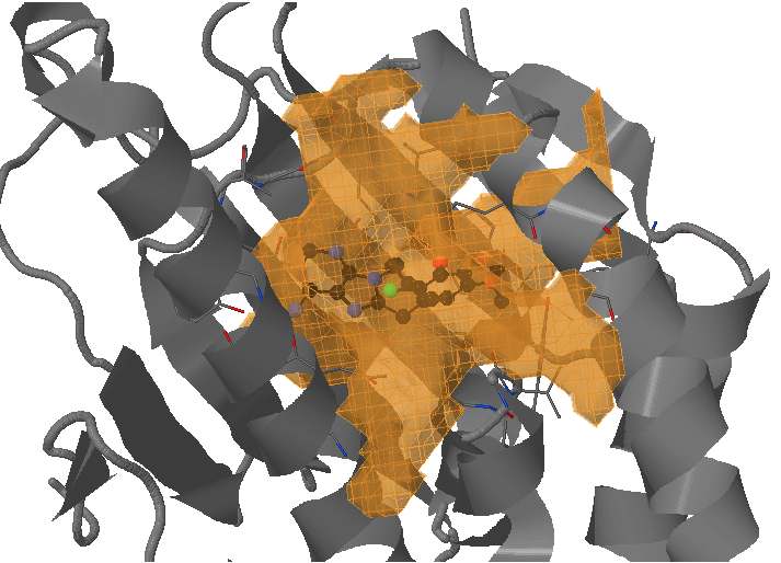
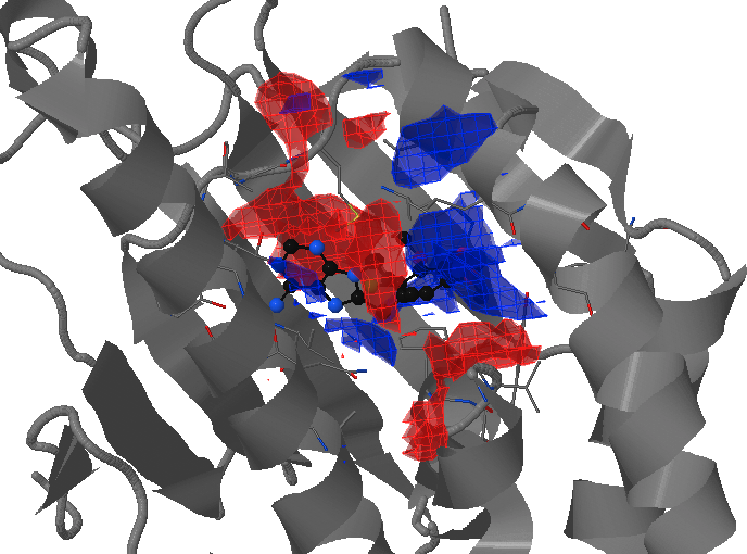
- Under Change JSmol View tab, the pocket from the reference strucutre (yellow) is displayed along with the reference structure. The appearing (red) and disappearing (blue) pocket regions from the trajectories can be displayed by selecting the respective occurance percentage. (See Fig.8, Fig.9)
In RIPlig, the perturbation procedure is applied not to the each protein residue, but to an artificial molecule placed in the binding pocket with repetitions starting with different positions of the molecule, which enables flexible regions of the binding site to be identified in a small number of MD simulations of several picoseconds duration. TRAPP-pocket results are generated seperately and in combination for all RipLig trajectories generated with LEU as the pseudo-ligand.
The results of TRAPP-pocket simulations for each Riplig trajectories can be viewed using the link: View Trj-LEU* results in JSmol that uses JSmol for visualization of transient pockets:
- Step 6: Analyzing TRAPP-pocket druggability results
- Snapshot 0 refers to the pocket druggability data obtained from the reference structure. (See Fig.11)
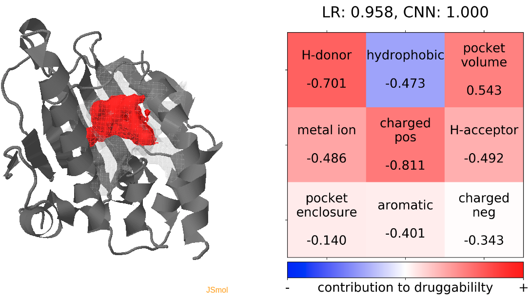
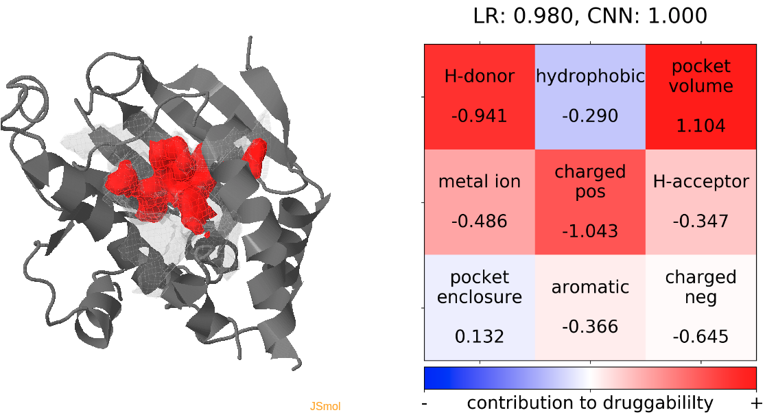
- The point with the lowest druggability score in the MD trajectory is at snapshot 3, where low hydrophobicity and pocket enclosure seem to be the reasons for lower druggability. (See Fig.12)
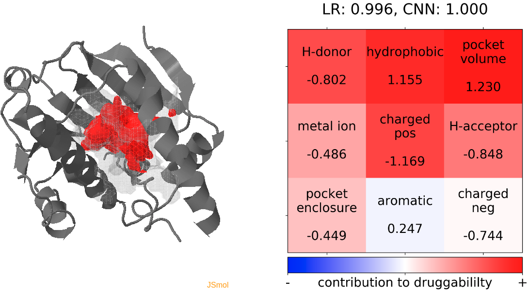
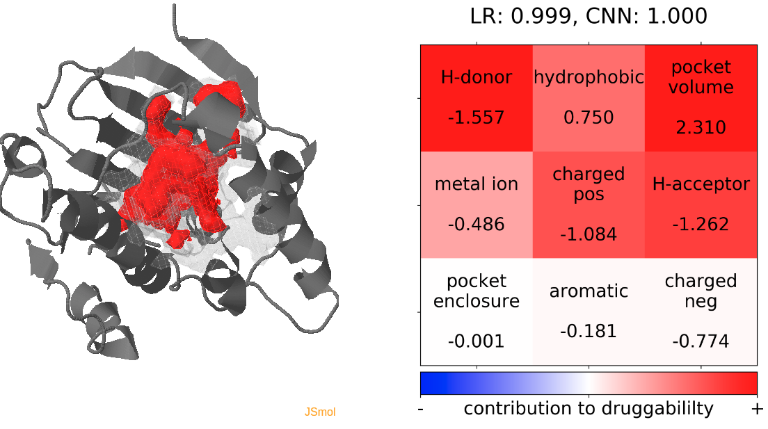
- The highest druggability score is at snapshot 32. The pocket volume and absence of H-donor and acceptors are the major contributors to druggability. (See Fig.13)
The results of TRAPP-pocket druggability are available under the Pocket characteristic tab.
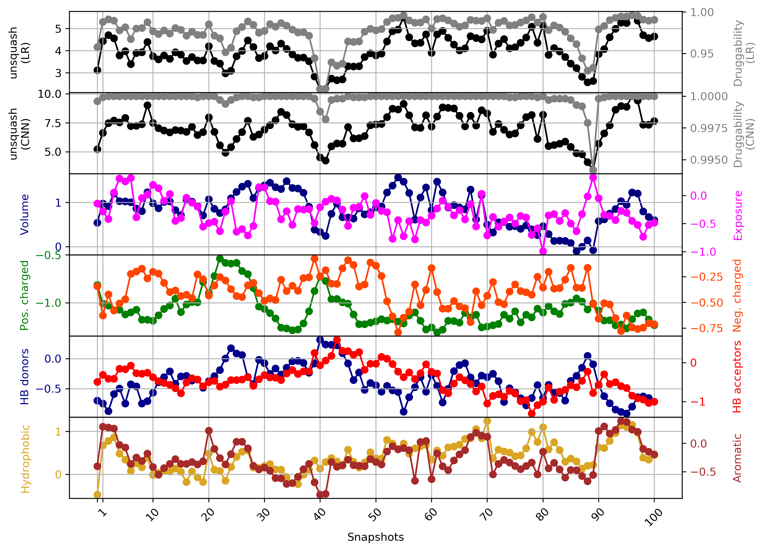
Click Pocket characteristics and druggability to visualize different physicochemical characteristics of the pocket and their contribution to the druggability (See Fig.16).
The druggability score of each frame in the MD trajectory was predicted by both TRAPP-LR and TRAPP-CNN models. The pocket druggability at a specific point in the MD trajectory can be analyzed by choosing the respective snapshot and clicking Load Result in Druggability information for selected snapshot section.
To analyze the cluster representatives results, click the link View Combined Trj- results in JSmol. The results of TRAPP-pocket druggability are available under the Pocket characteristic tab.


- Step 1: Uploading input data
You have to upload the reference protein and ligand structures (1UYD_protein.pdb and 1UYD_ligand.pdb), set the radius around the ligand center to 5 Angstroms, choose L-RIP method for simulation, and the number of L-RIP snapshots to be stored (100 is chosen in this example).
- Step 2: Preview and Starting simulations
On the next page Pocket analysis will be started with the following parameters you must be able to see the JSmol visualization of the reference structure, a ligand, as well as identification of the binding pocket.

- Step 3: View results of TRAPP-structure and TRAPP-analysis
Use the link View Analysis and View cluster representatives in JSmol

- Step 4: Run TRAPP-pocket
Click run PCA and run Clustering. Analysis will be done at the pocket occurrence of (%) of 25, 50. Check the Calculate Druggability box to compute pocket druggability. Click Launch TRAPP-pocket to start.

- Step 5: Understanding TRAPP-pocket results
- Under Change JSmol View tab, the pocket from the reference strucutre (yellow) is displayed along with the reference structure. The appearing (red) and disappearing (blue) pocket regions from the trajectories can be displayed by selecting the respective occurance percentage. (See Fig.8, Fig.9)
In L-RIP, perturbation is applied to the side chains of the binding site residues. TRAPP-pocket results are generated for all L-RIP trajectories that used different binding site residues for perturbation.
The results of TRAPP-pocket simulations for each L-RIP trajectories can be viewed using the link: View Trj-* results in JSmol that uses JSmol for visualization of transient pockets:
- Step 6: Analyzing TRAPP-pocket druggability results
- Snapshot 0 refers to the pocket druggability data obtained from the reference structure. (See Fig.11)
- The point with the lowest druggability score in the MD trajectory is at snapshot 41, where the presence of H-donor and acceptors in the binding pocket seems to be the reason for lower druggability. (See Fig.12)
- The highest druggability score is at snapshot 96. The pocket volume and high hydrophobicity are the major contributors to druggability. (See Fig.13)
The results of TRAPP-pocket druggability are available under the Pocket characteristic tab.
Click Pocket characteristics and druggability to visualize different physicochemical characteristics of the pocket and their contribution to the druggability (See Fig.10).
The druggability score of each frame in the MD trajectory was predicted by both TRAPP-LR and TRAPP-CNN models. The pocket druggability at a specific point in the MD trajectory can be analyzed by choosing the respective snapshot and clicking Load Result in Druggability information for selected snapshot section.
To analyze the cluster representatives results, click the link View Combined Trj- results in JSmol. The results of TRAPP-pocket druggability are available under the Pocket characteristic tab.